Can You Return All VLOOKUP Values?
October 16, 2018 - by Bill Jelen

VLOOKUP is a powerful function. But I often get a question in one of my Power Excel seminars from someone who wants to know if VLOOKUP can return all of matching values. As you know, the VLOOKUP with False as the fourth argument will always return the first match that it finds. In the following screenshot, cell F2 returns 3623 because it is the first match found for job J1199.
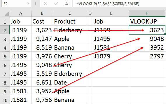
The question, then, can VLOOKUP return all of the matches?
VLOOKUP will not. But other functions can.
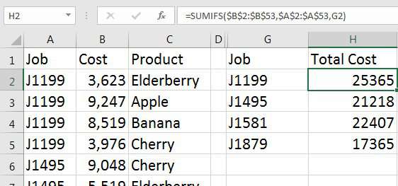
If you want to total all of costs from job J1199, you would use =SUMIFS($B$2:$B$53,$A$2:$A$53,G2),
If you have text values and want to join all of the results into a single value, you can use =TEXTJOIN(", ",TRUE,IF($A$2:$A$53=G2,$C$2:$C$53,"")). This formula only works in Office 365 and Excel 2019.

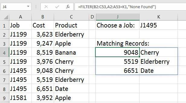
Or, you might need to return all of the results for a single job into a new range of the worksheet. A brand new =FILTER(B2:C53,A2:A53=K1,"None Found") function that is coming to Office 365 in 2019 will solve the problem:
Sometimes, people want to perform all of the VLOOKUPs and sum them. If your lookup table is sorted, you could use =SUM(LOOKUP(B2:B53,M3:N5)).
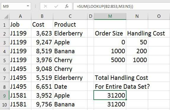
If you need to sum all VLOOKUPs with the Exact Match version of VLOOKUP, you will need to have access to Dynamic Arrays in order to use =SUM(VLOOKUP(B2:B53,M3:N5,2,TRUE)).
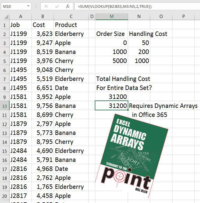
To learn more about Dynamic Arrays, check out Excel Dynamic Arrays Straight To The Point.
Watch Video
Video Transcript
Learn Excel From MrExcel, Podcast Episode 2247: Can You Return All VLookUp Values?
Hey. Welcome back to the MrExcel netcast. I’m Bill Jelen. Two questions came up in my seminar in Appleton, Wisconsin last week -- both related. They said, hey, how do we return all VLOOKUPs, alright? In this case, like J1199 has a bunch of matches and they, you know, want to return them all, and my first question whenever anyone asks me this is, well, what do you want to do with the matches? Are they numbers that you want to add up or is it text that you want to concatenate? And it's funny. The two questions in the same seminar, one person wanted to add them up and the other person wanted to concatenate the results.
So let's take a look at both of these. Check down in the YouTube description for a table of contents where you can jump to the other one if you want to see the result of the text.
Okay, so, first thing, if we want to add them all up, we're not going to use a VLOOKUP at all. We're going to use a function called SUMIF or SUMIFS which is going to sum everything that matches this item. So, SUMIFS. Here’s the numerical values that we want to sum and I'll press F4 to lock that down. That way, as I copy this down, it’s going to keep pointing to the same range, and then we want to go check and see if the JOB number in column A, again F4 there, is = to the value to the left of us -- in this case E2 -- and as we copy that down, we will see the TOTAL for each item. [SUMIFS($B$2:$B$53,$A$2:$A$53,E2)]
Let’s just do a little check here. J1199. The total is 25365. Alright. So, that's working. If it's numbers and you want to get all the numbers and add them up, switch over to SUMIF or SUMIFS, but if it's text, alright, now, this function is new in Office 365 in February 2017. So, if you have Excel 2016 or Excel 2013 or Excel 2010 or any of those older ones, you're not going to have this function. It's a function called TEXTJOIN. TEXTJOIN. This is another function from [Joe McDade – 01:50] who just brought us all those great dynamic array formulas at Ignite in 2018, and Joe made sure that TEXTJOIN would work with arrays, which is really great.
So, the delimiter here is going to be , SPACE, ignore EMPTY definitely. We want to ignore EMPTY here because we're going to generate a lot of empties in this next part, the IF statement. IF that item over an A2, F4, is = to this JOB number here, then I want the corresponding item from column C, F4, otherwise, I want “” like that. Close that IF statement. Close the TEXTJOIN. Do I have to press CONTROL+SHIFT+ENTER? No, I do not. It brings me all of the products that match like that, alright? So, returning all VLOOKUPs, if we want to sum them, yes, if we want to concatenate them, yes. [=TEXTJOIN(“,”,True,IF($A$2:$A$53=E2,$C$2:$C$53,“”))]
Alright, Now, there's one other possibility here when people ask me if they can return all VLOOKUPs. It might be an issue where we want to look up each of these costs here and figure out the HANDLING COST and then sum them all up. Like, I don't want to put a VLOOKUP here and a VLOOKUP here and a VLOOKUP here and a VLOOKUP here. I just want to do them altogether and, in that case, we're going to use the SUM function and then the old, old LOOKUP function. LOOKUP says that we're going to look up all of these values in column B. I don't need F4 here because I'm not copying it anywhere. ,. Here's our lookup table. ), close the SUM, and it goes out and does each individual VLOOKUP and then sums them all like that. [=SUM(LOOKUP(B2:B53,K3:L5))]
Well, hey. All of these topics are my book MREXCEL LIV: The 54 Greatest Tips Of All Time. Click that i in the top right-hand corner to learn more.
So, the question is can you return all VLOOKUPs? Well, sort of, but not actually using VLOOKUP. We’re either going to use SUMIF, TEXTJOIN, or SUM or LOOKUP to solve it.
Well, hey. I want to thank you for stopping by. We'll see you next time for another netcast from MrExcel.
You know, alright, I've been talking about these dynamic arrays for a week. I wanted to do one video where I didn't touch on dynamic arrays because I know a lot of people don't have them yet, but here we are. It's the outtake. You know, these aren't alphabetical. This would be so much better if we could sort them, and if you happen to have the new dynamic arrays, you could send this into the SORT function, SORT like this, and press ENTER, and now the results will be sorted like that.
You know, even this formula could get better with the dynamic arrays. The lookup requires you use the , TRUE. What if you wanted to use a , FALSE? We could change that to a VLOOKUP, lookup all of this text into that table , 2 ,. In this case, I am going to use TRUE but, in another case, you might use FALSE. CONTROL+SHIFT+ENTER. No. It's just going to work, alright? [=SUM(VLOOKUP(B2:B53,K3:L5,2,True))]
Dynamic Arrays coming out in early 2019 will solve so many problems.
Thanks for hanging out through the outtake here. We'll see you next time for another netcast from MrExcel.
Download Excel File
To download the excel file: can-you-return-all-vlookup-values.xlsx
When someone asks "Can VLOOKUP return all of the matches, the answer is No. But, there are many other functions that can do essentially the same thing.
Excel Thought Of the Day
I've asked my Excel Master friends for their advice about Excel. Today's thought to ponder:
"Normalize your data as you would have others normalize their data for you"
Title Photo: Ulises Baga on Unsplash
