Can I Save Formatting in a Template?
December 20, 2022 - by Bill Jelen

Problem: Every month, I have to change my pivot table formatting. Can I create a template to remember my favorite settings?
Strategy: The pivot table template concept is a frequent request as I do my Power Excel seminars. I predict that Microsoft won’t add this, because the people inside of Microsoft have embraced building a template using GetPivotData.
I first learned this technique from a former Microsoft staffer. It really is a cool way to improve your monthly reporting workflow. It will take an extra 15 minutes during the first month, but then it will save time in the future.
1. Build an ugly, unformatted pivot table with every field that you will need in your final report.
-
2. On a new worksheet, build a non-pivot table report shell that contains all of the formatting that you want to use.
3. Start in one cell of the report shell. Type an equals sign. Go to the pivot table and find the cell that contains the correct information. Click that cell and press Enter. Microsoft will build a
GETPIVOTDATAformula for you. Gotcha: The fields in the formula are hard-coded and can not be copied to other cells in the report.4. Edit the first formula to use labels in your report.
5. Copy the formula throughout your report.
Each month, the workflow becomes: Add new data to the data set. Refresh the ugly pivot table. Print the nicely formatted report that draws its numbers from the pivot table.
Here are some examples.
This figure shows a very ugly pivot table. Excel adds Plan+Actual in column D which is useless. There is no way to get Actuals for Jan through May and Plan for June through December without showing both fields for every month.
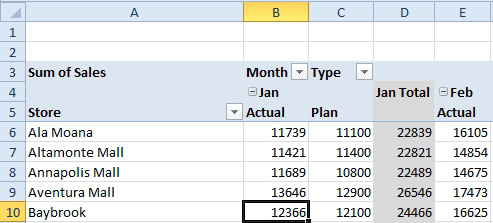
Typically, each month, you would create this pivot table, copy the table and paste as values. You would get rid of the columns you don’t need. You would resequence the stores in a geographic fashion. It would take half an hour to format the copied report.
Instead, build a report shell on a new worksheet. Format the report the way that you want it to be shown. If you want underlines and double-underlines, add them. If you want $ on row 1 and the total row, do that. If you want (gasp) a blank row, add it. You can do whatever you want, since this is not a pivot table. It is just Excel.
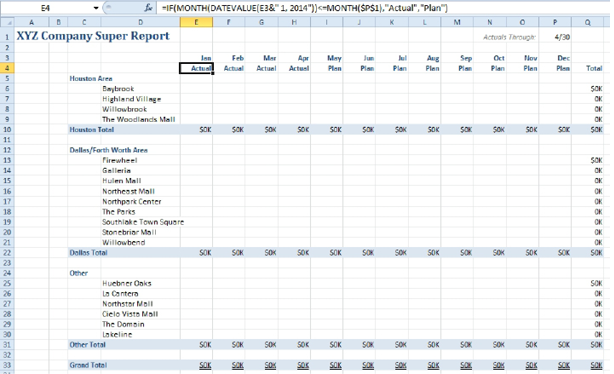
The first data cell in the report is for Baybrook Mall, January, Actuals. Choose that cell. Type an equals sign. Navigate to the pivot table worksheet and find the cell for Baybrook, January, Actual. Click on that cell and click OK.
Most of the time when Excel inserts a GETPIVOTDATA formula, it is an annoying side-effect of building a formula with a mouse. This time, it is crucial to building this report.
Gotcha: Most people are annoyed by Excel insert GETPIVOTDATA. See Calculations Outside of Pivot Tables to see how to turn this feature off. If someone has turned the feature off on your computer, you need to turn it back on.
The fundamental problem with the automatically generated GETPIVOTDATA function is that the label values are hard-coded in the formula instead of pointing to cells in the worksheet.
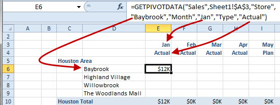
The accountants at Microsoft who use this trick regularly call this next step, “Parameterizing the Formula.” Change the three text values in the formula to point to cell addresses. Make sure to use the proper dollar signs. Replace Baybrook with $D6. Replace Jan with E$3. Replace Actual with E$4.
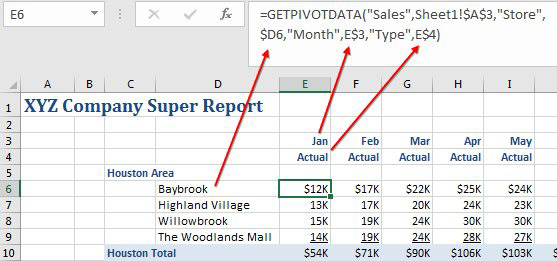
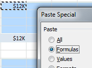
You can now copy that first formula and Paste Special Formulas to all the other report cells.
The result is a beautifully formatted report that is getting the data from the pivot table. Next month, add the May actuals, refresh the pivot table, and the report will update with new values.
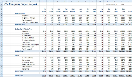
Additional Details: Cell P1 in the report is a date that I type manually each month. Formulas in row 4 use that date to show “Actual” or “Plan” based on the date. =IF(MONTH(DATEVALUE(E3&" 1, 2014"))<=MONTH($P$1),"Actual","Plan").
This article is an excerpt from Power Excel With MrExcel
Title photo by Nataliya Smirnova on Unsplash
