Calendar in Excel with One Formula (Array Entered, of Course!)

February 05, 2018 - by Bob Umlas

Create calendar in Excel with one formula by using array-entered formula.

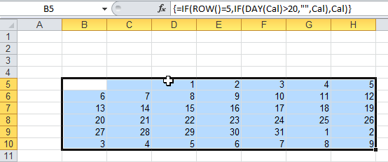
Look at this figure:

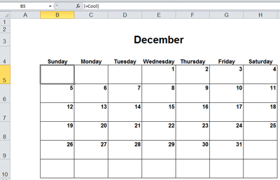
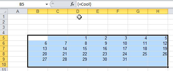
That formula, =Cool, is the same formula in every cell from B5:H10! Look:

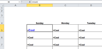
It was array-entered once B5:H10 was first selected. In this article you will see what is behind the formula.

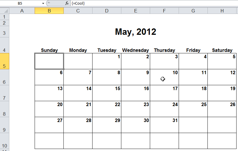
By the way, there's a cell which isn't shown yet which is the month to display. That is, cell J1 contains =TODAY(), (and I'm writing this in December) but if you change it to 5/8/2012, you would see:

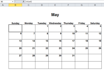
This is May, 2012. OK, definitely cool! Start from the beginning, and work your way up to this formula in the calendar and see how it works.

Also, assume that today is May 8, 2012.

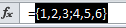
First, look at this figure:

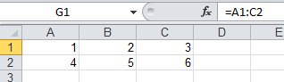
The formula doesn't really make sense. It would, if it were surrounded by =SUM, but you want to see what's behind the formula, so you will expand it by selecting it and pressing the F9 key.

The figure above becomes the figure below when the F9 key is pressed.

Notice that there's a semi-colon after the 3 - this indicates a new row. New columns are represented by a comma. So you are going to take advantage of that.

The number of weeks in a month varies, but no calendar needs more than six rows to represent any month, and of course, they all have seven days. Look at this figure:

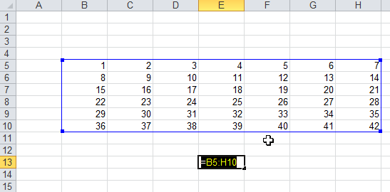
Manually enter the values 1 to 42 in B5:H10, and if you enter =B5:H10 in a cell and then expand the formula bar, you see what's shown here:

Notice the placement of the semicolons - after each multiple of 7 - indicating a new row. This is the start of the formula, but instead of such a long one, you can use this shorter formula. Select B5:H10. Type

={0;1;2;3;4;5}*7+{1,2,3,4,5,6,7}

as the formula, but do not press Enter.

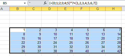
To tell Excel this is an array formula, you have to hold down Ctrl + Shift with your left hand. While holding Ctrl + Shift, press Enter with your right hand. Then, release Ctrl + Shift. For the rest of this article, this set of keystrokes will be called Ctrl + Shift + Enter.

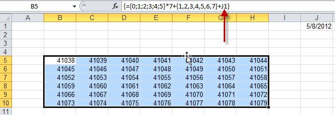
If you did Ctrl + Shift + Enter correctly, curly braces will appear around the formula in the formula bar and the numbers 1 to 42 would appear in B5:H10 as shown here:

Notice that you are taking the numbers 0 through 5 separated by semicolons (new row for each) and multiplying them by 7, effectively giving this:

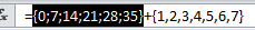
The vertical orientation of these values added to the horizontal orientation of the values 1 through 7 does yield the same values as shown. The expansion of this is identical to what you had before. Suppose now you add TODAY to these numbers?

Note: Editing an existing array formula is very tricky. Carefully, follow these steps: Select B5:H10. Click in the Formula Bar to edit the existing formula. Type +J1 but do not press Enter. To accept the edited formula, press Ctrl + Shift + Enter.

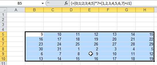
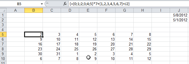
The result for May 8, 2012 is:

These numbers are serial numbers (the number of days since 1/1/1900). If you format these as short dates:

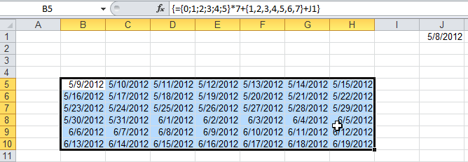
Clearly not right, but you will get there. What if you format these as simply "d" for the day of the month:

Almost looking like a month, but no month starts with the ninth of the month. Ah, here's one problem. You used J1 which contains 5/8/2012, and you really need to use the date of the first of the month. So suppose you put =DATE(YEAR(J1),MONTH(J1),1) in J2:

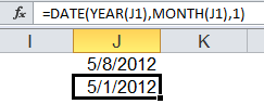
Cell J1 contains 5/8/2012 and cell J2 changes that to the first of the month of whatever is entered in J1. So if you change J1 in the formula of the calendar to J2:

Closer, but still not right. One further adjustment is needed, and that is you need to subtract the weekday of the first day. That is, cell J3 contains =WEEKDAY(J2). 3 represents Tuesday. So now if you subtract J3 from this formula, you get:

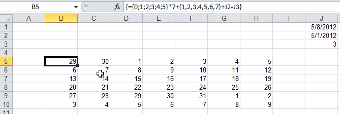
And that's actually right for May, 2012!

Okay, You are real close. What's still wrong is the 29 and 30 from April is showing up in the May calendar, and June 1 thru 9 is also showing up. You need to clear these.

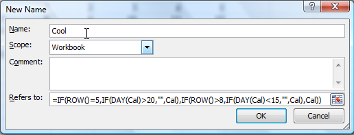
You can give the formula a name for easier reference. Call it "Cal" (not "cool" yet). See this figure:

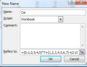
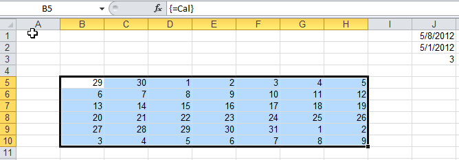
Then you can change the formula to simply be =Cal (still Ctrl + Shift + Enter):

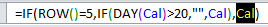
Now you can change the formula to read that if the result is in row 5 and the result is over 20, say, then that result should be blank. Row 5 will contain the first week of any month so you should never see any values over 20 (or any number over seven would be wrong - a number like 29 which you see in cell B5 of the figure above is from the previous month). So you can use =IF(ROW()=5,IF(DAY(Cal)>20,"",Cal),Cal):

First, notice that cells B5:D5 are blank. The formula now reads "if this is row 5, then if the DAY of the result is over 20, show blank".

You can continue to remove the low numbers at the end - next month's values. Here is how to do this easily.

Edit the formula and select the final reference to "Cal"

Begin typing IF(ROW()>8,IF(DAY(Cal)<15,"",Cal),Cal) to replace the final Cal.

The final formula should be

=IF(ROW()=5,IF(DAY(Cal)>20,"",Cal),IF(ROW()>8,IF(DAY(Cal)<15,"",Cal),Cal))

Press Ctrl + Shift + Enter. The result should be:

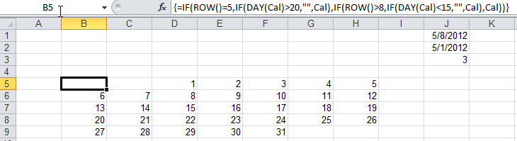
Two things left to do. You can take this formula and give it a name, "Cool":

Then use that in the formula shown here:

By the way, defined names are treated as if they are array-entered.

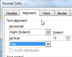
What's left to do is format the cells and put in the Days of the week and the name of the month. So you widen the columns, increase the row height, increase the font size, and align the text:

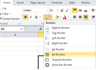
Then put borders around the cells:

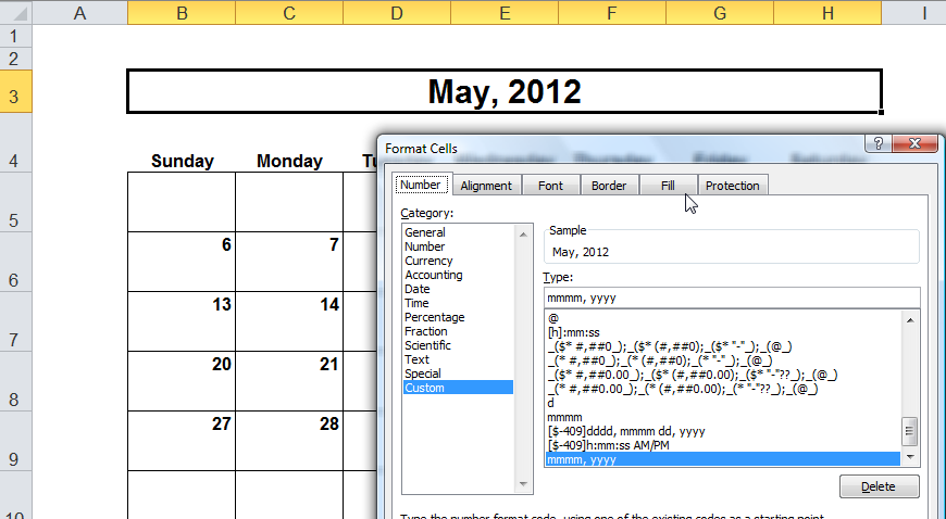
Merge and center the month & year and format it:

Then turn off gridlines, and voila:

Title Photo: Amber Avalona / Pixabay

This guest article is from Excel MVP Bob Umlas. It is from the book, Excel Outside the Box. To see the other topics in the book, click here.