Calculations Outside of Pivot Tables

January 30, 2023 - by Bill Jelen

Problem: I need to add a calculation in the grid outside of the pivot table that points to cells in the pivot table. Whenever I copy the formula, I get the exact same result!

Strategy: This started happening in Excel 2002. It is very annoying. I call it the GetPivotData bug.

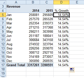
Here is how it happens. In the figure below, you’ve already grouped daily dates to months and years. Normally, you could add a calculated item to calculate growth rate as (2015/2014)-1, but calculated items are not allowed in grouped pivot tables. So, you went to cell D5, typed an equals sign, clicked on C5, typed a slash, clicked on B5, and pressed enter. The 14.54% is the correct growth rate. So, you then copied the formula down. Somehow, the growth rate for every month is identical.

Months Jan, Feb, and so on are in A5:A16 of this pivot table. Last year sales is in column B, this year sales in column C. Outside of the pivot table, a formula correctly calculates Growth for January as 14.54%. But when you copy this down, you get 14.54% for each row, which is not correct. — Figure 980. Sales went down in March 2015 from March 2014, there is no way that 14.54% growth is correct.

Select D5 and look in the formula bar. The formula there is =GETPIVOTDATA(“Revenue”, $A$3,”Date”,1, ”Years”, 2015) / GETPIVOTDATA( “Revenue”, $A$3,”Date”,1, ”Years”,2014)-1. There is no way that you typed any of that. You simply used the mouse when building the formula.

This also happens if you use the arrow keys. Equals Sign, Left, Slash, Left, Left, Minus, One, Enter will normally create a formula of =C5/B5-1, but in this case, you get the formula with two GETPIVOTDATA formulas.

What is GETPIVOTDATA and how did it get in your worksheet? The Excel team is hoping that you would see GETPIVOTDATA, then go find out what it is and learn to love it and use it all the time. But that is never what happens. Instead, people are annoyed by it.

As an aside, I spent eight years hating GETPIVOTDATA, but now I understand it and occasionally even use it. See “Can I Save Formatting in a Template” for an example of when you would want to use it.

The big question is how to enter a formula without getting the GETPIVOTDATA. One quick and easy way is to type the formula without using the mouse or the arrow keys. Just type =C5/B5-1. This creates a formula that will copy.

The other method is to permanently turn off the feature to generate GETPIVOTDATA. To do this, chose File, Options, Formulas. There is a checkbox for Use GetPivotData Functions For PivotTable References. Turn this off.

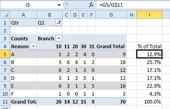
Additional Details: the other common problem with formulas outside of pivot tables is that they don’t deal well with the changing size of pivot tables. In Q1, six reason codes are found, so the % of Total formula points to G$11.

A somewhat complex pivot table. B1 filters the table to Q1. Reasons A through F appear in A5:A10. Branch numbers appear as column headings in B4:F4 with a Grand total column in G4. Column H is blank. A calculation outside the pivot table says Percent of Total and is using =G5/G$11. It is making the assumption that the Grand Total row will stay in row 11. — Figure 981. This works when there are six products.

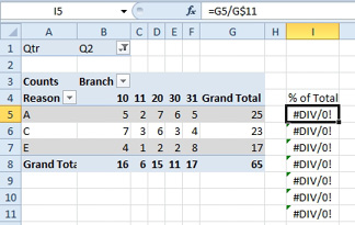
This doesn’t work anymore in Q2, when only three reason codes are found.

Disaster strikes when you change the Filter in B1 from Q1 to Q2. There are only three reason codes in column A, so the Grand Total is now in row 8. That means all of the calculations outside the pivot table that are pointing at G$11 are now returning Division by Zero errors. — Figure 982. The Grand Total moves from row 11 to row 8. Your formula is still dividing by G11.

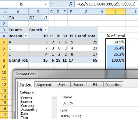
The solution is to use an Excel trick to return the last value from column G. Also, use a custom number format where the third zone is blank in order to hide any 0 values that appear below the table.

One solution is to change the formula to =G5/VLOOKUP(999,G$5:G$99,1). This hacked version of VLOOKUP returns the last number in column G. To prevent a bunch of zeroes from showing below the pivot table, use a Custom number format of 0.0%;-0.0%; The final semi-colon in that code creates an empty zone for zero values and they will not appear in the grid. — Figure 983. Two Excel tricks solve this problem.

This article is an excerpt from Power Excel With MrExcel

Title photo by Anant Jain on Unsplash