Calculated Fields in a Pivot Table

January 25, 2023 - by Bill Jelen

Problem: I need to include in a pivot table a calculation that is not in my underlying data. My data includes quantity sold, revenue, and cost. I would like to report gross profit and average price.

Strategy: You can add a calculated field to a pivot table. Follow these steps:

1. Build a pivot table with Product and Revenue columns.
2. The Calculated Field command is found under the Fields, Items, and Sets menu.

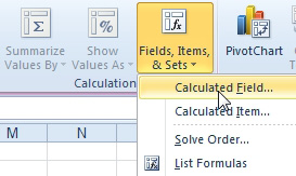
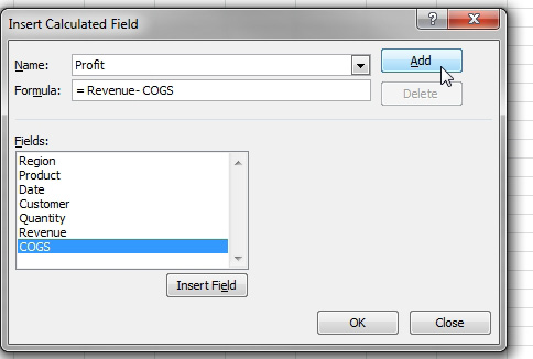
On the Pivot Table Analyze ribbon tab, open the Fields Items & Sets drop-down menu and choose Calculated Field. Other choices here are Calculated Item, Solve Order, and List Formulas. — Figure 962. Choose Calculated Field.

3. In the Insert Calculated Field dialog, type a field name such as Profit in the Name text box. In the Formula text box, type an equals sign. Double-click the Revenue entry in the Fields list. Type a minus sign. Double-click the COGS entry in the Fields List. The Formula text box should say =Revenue-COGS. Click the Add button to accept this formula.

In the Insert Calculated Field dialog, the name is Profit. The Formula is = Revenue - COGS — Figure 963. Add a new formula.

4. Add the following formula for GPPct: =Profit/Revenue.
5. Add the following formula for AveragePrice: =Revenue/Quantity.
6. Click OK to close the Insert Calculated Field dialog box.

Results: The resulting pivot table will include all the fields.

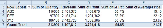
With Products in the rows area, the columns are Sum of Quantity, Revenue, Sum of Profit, Sum of GP Pct and Sum of Average Price — Figure 964. Excel adds the new fields to the pivot table.

Gotcha: The label Sum of GPPct is somewhat misleading, as is Sum of Average Price. In reality, Excel finds the sum of Revenue, finds the sum of Quantity, and then divides the values on the total line in order to get the average price. This makes calculated fields fine for any calculations that follow the associative law of mathematics. Having Excel do all the individual average prices and then sum them up would be impossible in a pivot table unless you are using Power Pivot.

You can rename the fields that have misleading headings. Simply click on the heading and type a new heading.

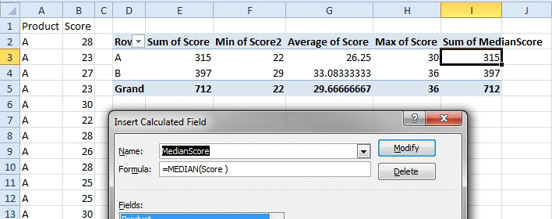
Gotcha: It is possible to use an Excel function in the Insert Calculated Field dialog. However, the function is applied to individual rows instead of using the population of matching rows. In the figure below, column I contains a calculated field of MEDIAN(Score). To calculate this, Excel takes the MEDIAN of cell B2. Of course, the median of B2 is the value from B2. They repeat this for each cell, then sum up the results. This is not a median at all. It is the same as the sum of the cells. To truly calculate a median, you will need Power Pivot.

A pivot table with Product in the rows area. Columns are Sum of Score, Min of Score, Average of Score, Max of Score. But the Calculated Field can't be right. The name is MedianScore. The formula is =MEDIAN(Score). In the pivot table, this shows as Sum of MedianScore, but the answers are all the same as the Sum of Score column — Figure 965. Using functions in calculated fields may not work as you want.

This article is an excerpt from Power Excel With MrExcel

Title photo by StellrWeb on Unsplash