Build a Better Top Five with A Filter Hack
January 02, 2023 - by Bill Jelen

Problem: Can you AutoFilter a pivot table? If you could turn on the AutoFilters and then filter to the top 6 items in column B, you would get the top five customers plus the real total.
Unfortunately, AutoFilter is greyed out when you are in a pivot table.
Strategy: Filter from the magic cell.
There is a strange loophole in the Filter logic. There are four ways to filter a data set. Microsoft greys out the Filter icon in the Data tab for three of those ways. They apparently missed the fourth method.
-
1. Create a pivot table with customers in the row labels.
2. Sort high to low by revenue.
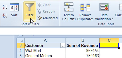
3. Select the cell to the right of the last heading. Below, this is cell C3. I call this cell the “magic cell” because it is an arcane cell that can filter the adjacent data set. It is so arcane, Microsoft forgets to gray out the filter command.
4. On the Data tab, click Filter.

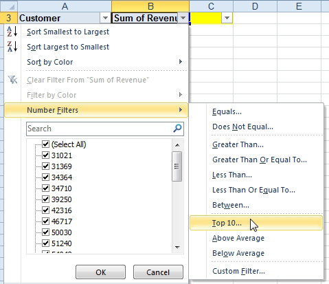
5. Open the dropdown in B3. You now have the AutoFilter choices instead of the Pivot filter choices. Choose Number Filters, Top 10.

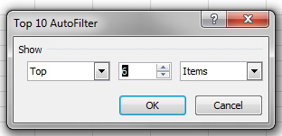
6. If you want to see the top five customers, choose 6 from the Top 10 AutoFilter dialog.

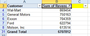
Result: the AutoFilter will show the largest item which is the Grand Total, plus the next five largest items, which are the customer totals. This figure is very similar to Figure 909, except this figure has the correct total for the entire data set.

Gotcha: Don’t forget the magic cell. In order to turn off the AutoFilter dropdowns, you have to go back and select cell C3. Otherwise, the Filter icon is greyed out.
Gotcha: This trick is clearly exploiting a bug in Excel. Don’t expect the AutoFilter to recalculate if you refresh the pivot table. Microsoft never expected that anyone would be able to AutoFilter a pivot table.
This article is an excerpt from Power Excel With MrExcel
Title photo by Tushar Rathour on Unsplash
