Budget versus Actual
August 31, 2017 - by Bill Jelen

Excel Data Model (Power Pivot) allows you to connect a large detailed data set of actuals to a top-level budget by using joiner tables.
Budgets are done at the top level – revenue by product line by region by month. Actuals accumulate slowly over time – invoice by invoice, line item by line item. Comparing the small Budget file to the voluminous Actuals data has been a pain forever. I love this trick from Rob Collie, aka PowerPivotPro.com.
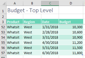
To set up the example, you have a 54-row budget table: one row per month per region per product.
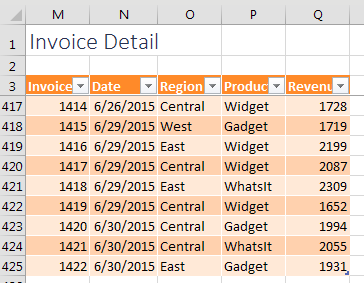
The invoice file is at the detail level: 422 rows so far this year.
There is no VLOOKUP in the world that will ever let you match these two data sets. But, thanks to Power Pivot (aka the Data Model in Excel 2013+), this becomes easy.
You need to create tiny little tables that I call “joiners” to link the two larger data sets. In my case, Product, Region, and Date are in common between the two tables. The Product table is a tiny four-cell table. Ditto for Region. Create each of those by copying data from one table and using Remove Duplicates.

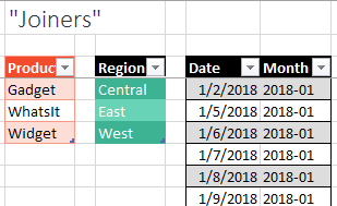
The calendar table on the right was actually tougher to create. The budget data has one row per month, always falling on the end of the month. The invoice data shows daily dates, usually weekdays. So, I had to copy the Date field from both data sets into a single column and then remove duplicates to make sure that all dates are represented. I then used =TEXT(J4,"YYYY-MM") to create a Month column from the daily dates.
If you don’t have the full Power Pivot add-in, you need to create a pivot table from the Budget table and check the box for Add This Data to the Data Model.

As discussed in the previous tip, as you add fields to the pivot table, you will have to define six relationships. While you could do this with six visits to the Create Relationship dialog, I fired up my Power Pivot add-in and used the diagram view to define the six relationships.
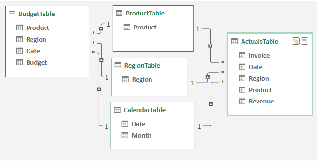
Here is the key to making all of this work: You are free to use the numeric fields from Budget and from Actual. But if you want to show Region, Product, or Month in the pivot table, they must come from the joiner tables!
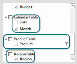
Here is a pivot table with data coming from five tables. Column A is coming from the Region joiner. Row 2 is coming from the Calendar joiner. The Product slicer is from the Product joiner. The Budget numbers come from the Budget table, and the Actual numbers come from the Invoice table.
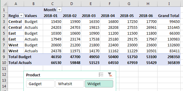
This works because the joiner tables apply filters to the Budget and Actual table. It is a beautiful technique and shows that Power Pivot is not just for big data.
Watch Video
- You have a small top-down budget data set
- You want to compare to a bottoms-up actuals data set
- The actuals might come from an invoice register
- The data model will let you compare these differing-size data sets
- Make both data sets into a Ctrl + T table
- For each text field that you want to report by, create a joiner table
- Copy the values and remove duplicates
- For dates, you can include dates from both tables and convert to month end
- Make the joiners be Ctrl + T tables
- Optional but helpful to name all five tables
- Create a pivot table from Budget and choose the Data Model
- Build a pivot table using Budget and Actual from the original tables
- All other fields must come from the joiner tables
- Add slicers by Product
- Create three relationships from Budget to Joiners
- Create three relationships from Actual to Joiners
- Tomorrow: how building relationships is easier with Power Pivot and DAX Formulas
Video Transcript
Learn Excel from MrExcel podcast, episode 2016 - Top-Down Budget vs Bottom-Up Actuals!
Hey, I'm podcasting this entire book, click that “i” on the top-right hand corner and follow the playlist.
Hey, I'm going to interrupt this, this is Bill Jelen from 15 minutes from now. I realize now this is an incredibly long podcast, and you're tempted just to click right through it, but let me just give you this short of it. If you're in Excel 2013, and you have ever had a small budget table and a massive actuals table, and you need to map them together, this is an amazing new ability that we have in Excel 2013, that not many people have explained, and you probably don't know about it. If this is you, you're in 2013, and you need to map these two data sets, take the time, maybe today, maybe tomorrow, maybe add it to the watch list, it's worth it, it's an amazing technique.
Alright, here's what we have, on the left-hand side we have a budget, this budget, it's done at the top-level, top-down, right for each product line, for each region, for each month, there's a budget. Not many records here, count of 55, on the right-hand side we're trying to compare this to actuals. The actuals are coming from an invoice register, so we have Region, Product, and Revenue, but they’re individual invoices, a lot more data here, we’re already halfway through the year, and I already have 423 records. Alright, so how do you map these 55 to these 423? Might be tough to do with VLOOKUP, you'd have to summarize first, but thankfully in Excel 2013, the data model makes this really, really easy. What we need to allow this big massive table to communicate with this tiny table are intermediaries, I call them joiners. Tiny little tables, Product, Region, and Calendar, we're going to join the budget to these three tables, we’re going to join the actual to these three tables, and miraculously the Pivot table will work. Alright, so here's how we do that.
First off I need to create the joiners, so I take this Product field from column A, and I copy it over to column F, and then Data, Remove Duplicates, click OK, and we're left with a tiny little table, 1 heading 3 rows. Same thing for Region, take the regions, Ctrl+C, go over to column G, Paste, Remove Duplicates, click OK, 3 rows 1 header, alright. Now for the dates, the dates are not the same, these are month ending dates, they're actually stored as month ending dates, and these are weekdays. I'm going to take both lists, Ctrl+C the second list and paste it here, Ctrl+V, then I'm going to take the shorter list, copy that, and paste it down below, alright. And it's really annoying that, even though these are stored as dates, they're appearing as months, and Remove Duplicates won't see them as the same. So before I use Remove Duplicates, I have to change it to a short date. Choose that data, Data, Remove Duplicates, click OK, and then a little sort here to get it to work.
Alright, now I don't want to report by daily date, so I'm going to add a column here, a lookup column that says Month, and this will be equal EOMONTH that date, ,0, which will get us out to the end of the month. It will format that as short date, and copy that down, alright. Now, we need to make each of these into a Ctrl+T table, so from here Ctrl+T, My table has headers, beautiful. The small ones, it doesn't realize those are headers up there, so we have to make sure to check mark that and Ctrl+T, alright, and they call these tables Table1, Table2, Table3, really boring names, right? So I'm going to rename these and call it the BudTable, the ProdTable, RegTable, my CalTable, and then the ActTable, alright.
We start from the very first table, and by the way we're not going to use PowerPivot today, we’re going to do all this with the data model. So, Excel 2013 or newer, you have this Insert, PivotTable, we're going to check the box for “Add this data to the Data Model”, click OK, and we get our field list with the magic All button, that lets me choose from all five tables in the workbook, Actual, Budget, Calendar, Product, Region. Alright, so the numbers are going to come from the Budget table, I'll put the budget in there, and from the Actual table I'll put the actual in there, but then here's the thing for the rest of the Pivot table. Any other text fields that we're going to put in the row area or the column area or as slicers, they have to come from the joiners, they have to come from those tables between the tables.
Alright, so from the Calendar table we'll take that Month field and put it across the top, we’re going to ignore other relationships right now. I will be creating the relationships, but I want to create them all at once. And the Region table, put the regions down the side. I could put products down the side, but I'm actually going to use the Product table as a slicer, so Analyze, Insert Slicer, again you have to go to All if you haven't used the Product table yet. So go to All, and you'll see that the Product is available to create as slicer from the products, like that. Alright now, at this point we haven't created relationships, so all of these numbers are wrong. And the relationships we have to create, we have to create 3 tables from this little budget table, one to the products, one to regions, one to calendar, that’s 3 relationships. And then we have to create relationships from the Actual table to the Product region in Calendar, so a total of 6 tables. And yes, this would definitely be easier if we had PowerPivot, but we don't or let's assume we don't.
And so I'm going to use the old-fashioned way, the Create dialogue here, where we have the Budget table on the left, and we're going to use the Region field and relate that to the Region table, the Region field. Alright, 1/6 are created. I'll choose Create, again from the Budget table we go to the Product, and then link that to the Product table, to the Product, click OK. From the Budget table the Date field, we go to the Calendar table, and the Fate field, click OK, we're halfway there, alright. From the Actuals table, we go Region, to the Region table, click OK, from the Actuals table to the Product, and from the Actuals table to the Calendar. I'm actually going to take the Values and make it go down the side, alright. Design, Report Layout, Show in Tabular Form to get a view that I prefer, Repeat All Item Labels, alright, this is absolutely amazing! Now we have this tiny little table, a 50-some records in this table of hundreds of records, and we've created a single Pivot table thanks to the Data Model. For each where we can see the Budget, we can see the Revenue, it's broken out by Region, it's broken out by Month, and it's sliceable by Product.
Now this concept came to me from Rob Collie who runs Power Pivot Pro, and Rob has created a lot of books out there, his latest one is “Power Pivot and Power BI”. I think this one was actually in the “Power Pivot Alchemy” book, it's the one that I saw this and I said “Well this, even though I don't have millions of rows to report through Power Pivot, this is one that would have made a HUGE difference in my life, having two data sets of mismatched sizes, and needing to report from both of them.” Well this example and many others are in this book, I will eventually get the entire book podcast, that looks like it's going to take two and a half months. But you can get the whole book today, same time, go there, buy the book, $10 for the e-book, $25 for the print book, and you can have all those tips at once.
Alright, a really long episode here: we have a small top-down Budget and a bottoms up Actual, they're different sizes, but using the data model in Excel 2013... And by the way if you're in 2010, you could, in theory, do this by getting the Power Pivot add-in, and go through all these steps back in 2010. Make both datasets into a Ctrl+T table, and then join your tables for anything you want to report on, in the row label, or the column label, or the slicers, so copy those values over and Remove Duplicates for the dates. I actually took values from both tables, because there were some unique values in each, and then I used the EOMONTH to get out there, make those joiner tables be controlled tables. It's optional, but I named all 5 tables, because easier when you're setting up those relationships, rather than having be called Table1, Table2, Table3.
And so, start from the Budget table, Insert, PivotTable, check the box for Data Model, and then building a Pivot table using Budget and Actual. Everything else comes from the joiner tables, so Region and Month in the row and column area, slicers came from the Product table. And then we had to create 3 relationships from the Budget to the joiners, 3 relationships from the Actual to the joiners, and we have an amazing Pivot table. Now tomorrow we'll take a look at using the Power Pivot tab and creating some additional calculations. So all of this is possible, it's when we want to insert a calculated field, that's when you have to pay the extra $2 a month to get the Pro Plus version of Office 365.
Well hey, thanks to Rob Collie from Power Pivot Pro for this tip, and thanks to you for stopping by, we'll see you next time for another netcast from MrExcel!
Download File
Download the sample file here: Podcast2016.xlsx
Title Photo: stevepb / pixabay
