Avoid Errors Using IFERROR

April 01, 2022 - by Bill Jelen

Problem: I’ve written a brilliant formula. Sometimes, due to the incoming data, the formula generates an error. How can I suppress the errors?

Strategy: Starting in Excel 2007, Excel offers the amazing IFERROR function. Don’t confuse this with the =ISERROR(), =ISERR(), =ISNA() functions. This new IFERROR function is very cool.

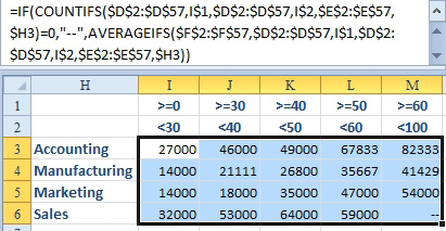
Before Excel 2007, to head off errors, you would have to test for any of the conditions that would cause an error. This might mean taking the very long formula from Figure 407 and making it insanely long:

=IF(COUNTIFS($D$2:$D$57,I$1,$D$2:$D$57,I$2,$E$2:$E$57,$H3)=0,”--”,AVERAGEIFS($F$2:$F$57,$D$2:$D$57,I$1,$D$2:$D$57,I$2,$E$2:$E$57,$H3))

There are 20 cells in Figure 407, and 19 of them are working just fine. Yet, this formula will force Excel to do a complete SUMIFS before it can figure out if it should put -- or go on to calculate the AVERAGEIFS. This a huge amount of complexity just to zap one #DIV/0! error.

The hard way to prevent the Division by 0 is IF the COUNTIFS equals zero, then put -- otherwise do the AVERAGEIFS. — Figure 408. Before Excel 2007, error handling was slow and complex.

Handling errors with IFERROR is dramatically easier. Say that you have any formula. Edit the formula. Type IFERROR( after the existing equals sign. Go to the end of the formula, type a comma, then what you want to have happen in case there is an error, then the closing parenthesis.

Say that you had a formula of =Formula.

To replace errors with a zero, use =IFERROR(Formula,0)
To replace errors with --, use =IFERROR(Formula,”--”)
You can specify another formula: =IFERROR(Formula,OtherFormula).

Think about most data sets where some errors occur. You probably have more than 95% of the cells that calculate without an error and less than 5% that generate errors. The IFERROR function is smart enough to try the first calculation and only move on to the second argument when it gets an error. This will be a drastic time savings when you don’t have to use =IF(ISNA(VLOOKUP()),”--”,VLOOKUP()) anymore.

The easy way to prevent the Division by zero error is to wrap the AVERAGEIFS in =IFERROR(formula,"-") — Figure 409. IFERROR simplifies error checking.

Additional Information: Excel 2013 adds the =IFNA() function. Say that you want to catch any VLOOKUP functions that return #N/A, but you want to allow any underlying DIV/0 errors to show through. The IFNA in Excel 2013 will only convert #N/A to the alternate value.

This article is an excerpt from Power Excel With MrExcel

Title photo by Jose Aragones on Unsplash