Add Visual Filters to a Pivot Table or Regular Table

January 10, 2023 - by Bill Jelen

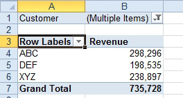
Problem: Excel 2007 added the ability to select multiple items from a filter. But when I do this, it uses the ambiguous (Multiple Items) heading. When I print this report, no one knows which customers are in the report.

The Customer filter in the pivot table is set to (Multiple Items). The big question: Which items? — Figure 925. When you select two customers from the filter dropdown, you can’t see which customers are selected.

Strategy: That addition in Excel 2007 was a first step towards the full visual filters called Slicers in Excel 2010. You can see which fields are included or not included. If you have Excel 2013, you can use Slicers on your Ctrl+T table in addition to Pivot Tables.

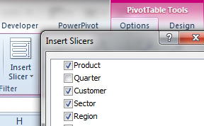
After building a pivot table, choose Insert Slicers. You can choose as many fields as you want from the current pivot table.

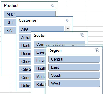
On the Pivot Table Tools Analyze tab, choose Insert Slicer. In the Insert Slicers dialog, choose Product, Customer, Sector, and Region. — Figure 926. Select fields to use as visual filters.

Initially, Excel tiles all of the slicers and shows them with one column. Here is the default arrangement of four slicers.

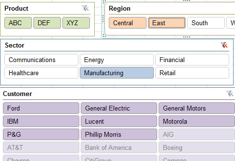
The four slicers are tiled from top left to bottom right. — Figure 927. By default, the slicers are tiled.

You will want to rearrange and resize the slicers. You can move and resize the slicers. In the Slicer Tools ribbon tab, use the Columns spinbutton to add more columns to a slicer. As you can see below, product and region can fit in a single row by increasing the number of columns to three or four.

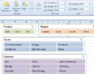
Drag the slicers into new positions so you can see all of each slicer. Change the colors (Product as green, Region as Orange, Sector as Blue, Customer as Purple). Using the Slicer Tools ribbon, change the number of Columns for each slicer: Product is 3 columns. The other slicers are four columns. — Figure 928. Rearrange and resize the slicers.

I also use a different color for each slicer. This is controlled in the Slicer Tools ribbon tab as well.

Once you have the slicers, you can choose from any slicer. The pivot table will update to reflect the filters. The other slicers will also update. Below, after choosing Manufacturing in the East & Central regions, several non-manufacturing customers are “greyed out” at the bottom of the customer slicer.

After choosing Region = Central or East and then Sector = Manufacturing, the Customer slicer is cross-filtered. The Customer slicer shows 8 customers in purple and the remaining customers in a greyed-out purple. The greyed out customers did not have any sales in Central or East Manufacturing. — Figure 929. AIG is greyed out since it isn’t in the Manufacturing sector.

Gotcha: I found it tough to select multiple items from one slicer. If you happen to need adjacent items, you can click on one and drag across to the next item. But, if you want to select ABC and XYZ, you have to choose ABC, then Ctrl+Click XYZ.

This article is an excerpt from Power Excel With MrExcel

Title photo by Afif Ramdhasuma on Unsplash