Xlookup or similar

[djjamesp]

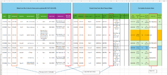
Hi all, I'm trying to get the following sheet to return one of four possible outcomes, but no matter what I try it doesn't quite work. I've also tried to upload the mini sample sheet but due to work restrictions on my works laptop it will not allow me to install the add-in.

- C5:8000 and M5:8000 will both contain the same unique ref numbers, but on different rows
- Column J on the same row as column C will have a yes, no or N/A value
- Column R on the same row as Column M will contain a value or blank
- If column J is Yes and M has a value return 'OKAY'
- If column J is No or N/A and M has a value return 'TECH ERROR'
- If column J is Yes and M has no value return "ENGINEER FAILED'
- if column J is No and M has no value return 'NOT REQUIRED'

examples
- C5 & M9 match, J5=Yes & M=Yes this will return 'OKAY'
- C12 & M14 match, J12=No & M14=No this will return 'NOT REQUIRED'

The two ways I went about this so far are

=IF(AND(COUNTIF(M5:M$8000, C1) > 0, J1 = "Yes", NOT(ISBLANK(INDEX(R:R, MATCH(C1, M:M, 0))))), "OKAY", IF(AND(COUNTIF(M:M, C1) > 0, J1 = "No", NOT(ISBLANK(INDEX(R:R, MATCH(C1, M:M, 0))))), "TECH ERROR", IF(AND(COUNTIF(M:M, C1) > 0, J1 = "Yes", ISBLANK(INDEX(R:R, MATCH(C1, M:M, 0)))), "ENGINEER FAILED", IF(AND(COUNTIF(M:M, C1) > 0, J1 = "No", ISBLANK(INDEX(R:R, MATCH(C1, M:M, 0)))), "NOT REQUIRED", ""))))

and

=IFERROR( IF(J5="Yes", IF(NOT(ISBLANK(XLOOKUP(C5, M$5:M$8000, R$5:R$8000, "", 0))), "OKAY", "ENGINEER FAILED"), IF(NOT(ISBLANK(XLOOKUP(C5, M$5:M$8000, R$5:R$8000, "", 0))), "TECH ERROR", "NOT REQUIRED") ), ""

I've spent a couple of days on this so far and I'm struggling!

Any help is greatly appreciated

Thanks in advance

James

 

[Peter_SSs]

examples
- C5 & M9 match, J5=Yes & M=Yes this will return 'OKAY'
- C12 & M14 match, J12=No & M14=No this will return 'NOT REQUIRED'

The above does not make sense to me since you said (& your image confirms) that M contains ref numbers, not Yes or No

M5:8000 will both contain the same unique ref numbers

However, perhaps this is the sort of thing you are after?

24 10 30.xlsm
	C							J	K		M					R							Y	Z
5	Ref 1							Yes			Ref 2					3								ENGINEER FAILED
6	Ref 2							No			Ref 3													TECH ERROR
7	Ref 3							N/A			Ref 4					2								NOT REQUIRED
8	Ref 4							No			Ref 5					5								TECH ERROR
9	Ref 5							Yes			Ref 1													OKAY
10	Ref 6							Yes			Ref 6					5								OKAY
Outcomes

Cell Formulas
Range	Formula
Z5:Z10	Z5	=LET(m,XLOOKUP(C5,M$5:M$10,R$5:R$10),IF(J5="Yes",IF(m="","ENGINEER FAILED","OKAY"),IF(m="","NOT REQUIRED","TECH ERROR")))

 

[djjamesp]

@Peter_SSs that looks pretty good, I'll give that a try and see how that works in my sheet, thank you!

 

[djjamesp]

I've played with the syntax a little but it still doesn't give the correct results, I've simplified my example spreadsheet down significantly and I realised the error of my original example - I hadn't updated the 'results' to reflect how I wanted it to display, (sincere apologies, I can see why that confused anyone) please see the example below of what I want to achieve.

Column M is the starting reference point

 

[Peter_SSs]

Column M is the starting reference point

We didn't have that information before.
I think that my previous formula was basically correct but it put the results on the row with the Job Number in column C rather than on the row with the job number in column M. The change makes the formula bit simpler.
Also, I did use col R instead of Q so have fixed that
Another change is that you have changed from "TECH ERROR" to "TECH FAILED"
Given all that, see how this version goes.

24 10 30.xlsm
	C							J	K		M	N	O	P	Q							X	Y	Z
5	SR/19200							Yes			SR/19207													ENGINEER FAILED
6	SR/19201							No			SR/19206				C17									TECH FAILED
7	SR/19202							Yes			SR/19205				B07									OKAY
8	SR/19203							No			SR/19204													NOT REQUIRED
9	SR/19204							No			SR/19203													NOT REQUIRED
10	SR/19205							Yes			SR/19202				A01									OKAY
11	SR/19206							No			SR/19201													NOT REQUIRED
12	SR/19207							Yes			SR/19200													ENGINEER FAILED
Outcomes (2)

Cell Formulas
Range	Formula
Z5:Z12	Z5	=IF(XLOOKUP(M5,C$5:C$12,J$5:J$12)="Yes",IF(Q5="","ENGINEER FAILED","OKAY"),IF(Q5="","NOT REQUIRED","TECH FAILED"))

 

[djjamesp]

That is perfect, apologies for all the confusion - this is a live spreadsheet and I'm working on it constantly adding and removing things so some of the cell references have got mixed up. Wow, you don't know how much relief that's given me! Thank you so much!!

 

[Peter_SSs]

You're welcome. Thanks for the follow-up.