Hi,
I’m creating an interactive dashboard containing pivot charts for different product sales at my work. The dashboard also contains a slicer that controls ALL charts in the dashboard since all are present and made from the data model.
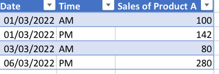
Within my original excel file, I’ve got a table that has got sales for product A against the date and time of when the sale was made (see screenshot of small sample data from this table). The table only contains dates where a sale for Product A has been made so there is no record in the table when a sale of product A has not been made.
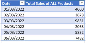
I’ve got another table that has got sales for all of the different products against the dates when these sales were made (see screenshot of sample data from this table as well).
My aim is to represent Percentage of Total Sales made by Product A broken down by date and since my dashboard is interactive, I’d like to give my user the option of viewing aggregated data for month or years as well using pivot table date grouping. So as an example, for 01/03/2022, this would be (100+142)/4000 * 100. This would be perfectly straightforward to do if the data were all in one table as I’d just have to use a calculated field in pivot table to calculate this.
However, since the data is in two separate tables, I have had to create a relationship between the two tables using the DATE field of the two tables. Unfortunately, since I now have to create the pivot table/chart from the data model, I can no longer use a calculated field.
Is there any workaround that I can implement to achieve this? Any help would be greatly appreciated!
Please see below things I’ve already tried:
I tried creating a new column in the total sales of ALL products table and used a SUMIF function to sum product A sales. Then, in the data model, I created a calculated field to calculate the percentage for each date. Although this works for individual dates, it doesn’t work for aggregated monthly percentages because excel sums up the percentages rather than doing (sum all sales for the month)/(sum product A sales for the month) * 100.


