VLookup Match Function for Range

[Steveym]

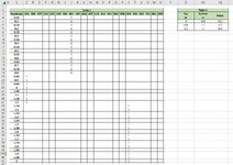
Good morning, I have a table I would like to populate automatically if the values lie within a specific range.

In the example attached, I would like to populate Table 1 with data from the depth ranges from Table 2.

For example in Table 2 between 0 and 0.8 the value is '401' so this has populated correctly in the '401' column across the corresponding depth range in Table 1.

Many thanks for any help.

Steven

 

[Special-K99]

Try (somewhat tested) in B4 and copy across and down the sheet

=SUMPRODUCT(($A4>=$Z$5:$Z$7)*($A4<$AA$5:$AA$7)*(B$3=INDEX($AB$5:$AB$7,MATCH($A4,$Z$5:$Z7,1),1)))

 

[Steveym]

Try (somewhat tested) in B4 and copy across and down the sheet

=SUMPRODUCT(($A4>=$Z$5:$Z$7)*($A4<$AA$5:$AA$7)*(B$3=INDEX($AB$5:$AB$7,MATCH($A4,$Z$5:$Z7,1),1)))

Excellent, many thanks!

 

[Peter_SSs]

Excellent, many thanks!

Are you sure? Doesn't that formula include some incorrect '1' values (orange below) and miss some required '1' values (green) compared to your image?

23 08 09.xlsm
	A	B	C							J									S	T	U	V	W	X	Y	Z	AA	AB
3			201							401									509	520	525	701	801	805
4		0.05	0							1									0	0	0	0	0	0
5		0.1	0							1									0	0	0	0	0	0		0	0.8	401
6		0.15	0							1									0	0	0	0	0	0		0.8	1.2	201
7		0.2	0							1									0	0	0	0	0	0		1.2	2	509
8		0.25	0							1									0	0	0	0	0	0
9		0.3	0							1									0	0	0	0	0	0
10		0.35	0							1									0	0	0	0	0	0
11		0.4	0							1									0	0	0	0	0	0
12		0.45	0							1									0	0	0	0	0	0
13		0.5	0							1									0	0	0	0	0	0
14		0.55	0							1									0	0	0	0	0	0
15		0.6	0							1									0	0	0	0	0	0
16		0.65	0							1									0	0	0	0	0	0
17		0.7	0							1									0	0	0	0	0	0
18		0.75	0							1									0	0	0	0	0	0
19		0.8	1							0									0	0	0	0	0	0
20		0.85	1							0									0	0	0	0	0	0
21		0.9	1							0									0	0	0	0	0	0
22		0.95	1							0									0	0	0	0	0	0
23		1	1							0									0	0	0	0	0	0
24		1.05	1							0									0	0	0	0	0	0
25		1.1	1							0									0	0	0	0	0	0
26		1.15	1							0									0	0	0	0	0	0
27		1.2	0							0									1	0	0	0	0	0
28		1.25	0							0									1	0	0	0	0	0
29		1.3	0							0									1	0	0	0	0	0
30		1.35	0							0									1	0	0	0	0	0
31		1.4	0							0									1	0	0	0	0	0
32		1.45	0							0									1	0	0	0	0	0
33		1.5	0							0									1	0	0	0	0	0
34		1.55	0							0									1	0	0	0	0	0
35		1.6	0							0									1	0	0	0	0	0
36		1.65	0							0									1	0	0	0	0	0
37		1.7	0							0									1	0	0	0	0	0
38		1.75	0							0									1	0	0	0	0	0
39		1.8	0							0									1	0	0	0	0	0
40		1.85	0							0									1	0	0	0	0	0
41		1.9	0							0									1	0	0	0	0	0
42		1.95	0							0									1	0	0	0	0	0
43		2	0							0									0	0	0	0	0	0
Table (2)

Cell Formulas
Range	Formula
C4:C43,J4:J43,S4:X43	C4	=SUMPRODUCT(($B4>=$Z$5:$Z$7)*($B4<$AA$5:$AA$7)*(C$3=INDEX($AB$5:$AB$7,MATCH($B4,$Z$5:$Z$7,1),1)))

Since you have Excel 365, would this work for you instead?

23 08 09.xlsm
	B	C							J									S					X	Y	Z	AA	AB
1
2
3		201							401									509					805
4	0.05								1
5	0.1								1																0	0.8	401
6	0.15								1																0.8	1.2	201
7	0.2								1																1.2	2	509
8	0.25								1
9	0.3								1
10	0.35								1
11	0.4								1
12	0.45								1
13	0.5								1
14	0.55								1
15	0.6								1
16	0.65								1
17	0.7								1
18	0.75								1
19	0.8								1
20	0.85	1
21	0.9	1
22	0.95	1
23	1	1
24	1.05	1
25	1.1	1
26	1.15	1
27	1.2	1
28	1.25																	1
29	1.3																	1
30	1.35																	1
31	1.4																	1
32	1.45																	1
33	1.5																	1
34	1.55																	1
35	1.6																	1
36	1.65																	1
37	1.7																	1
38	1.75																	1
39	1.8																	1
40	1.85																	1
41	1.9																	1
42	1.95																	1
43	2																	1
Table

Cell Formulas
Range	Formula
C4:C43,J4:J43,S4:S43,X4:X43	C4	=IF(XLOOKUP($B4,$AA$5:$AA$7,$AB$5:$AB$7,,1)=C$3,1,"")

 

[Steveym]

Are you sure? Doesn't that formula include some incorrect '1' values (orange below) and miss some required '1' values (green) compared to your image?

23 08 09.xlsm
	A	B	C							J									S	T	U	V	W	X	Y	Z	AA	AB
3			201							401									509	520	525	701	801	805
4		0.05	0							1									0	0	0	0	0	0
5		0.1	0							1									0	0	0	0	0	0		0	0.8	401
6		0.15	0							1									0	0	0	0	0	0		0.8	1.2	201
7		0.2	0							1									0	0	0	0	0	0		1.2	2	509
8		0.25	0							1									0	0	0	0	0	0
9		0.3	0							1									0	0	0	0	0	0
10		0.35	0							1									0	0	0	0	0	0
11		0.4	0							1									0	0	0	0	0	0
12		0.45	0							1									0	0	0	0	0	0
13		0.5	0							1									0	0	0	0	0	0
14		0.55	0							1									0	0	0	0	0	0
15		0.6	0							1									0	0	0	0	0	0
16		0.65	0							1									0	0	0	0	0	0
17		0.7	0							1									0	0	0	0	0	0
18		0.75	0							1									0	0	0	0	0	0
19		0.8	1							0									0	0	0	0	0	0
20		0.85	1							0									0	0	0	0	0	0
21		0.9	1							0									0	0	0	0	0	0
22		0.95	1							0									0	0	0	0	0	0
23		1	1							0									0	0	0	0	0	0
24		1.05	1							0									0	0	0	0	0	0
25		1.1	1							0									0	0	0	0	0	0
26		1.15	1							0									0	0	0	0	0	0
27		1.2	0							0									1	0	0	0	0	0
28		1.25	0							0									1	0	0	0	0	0
29		1.3	0							0									1	0	0	0	0	0
30		1.35	0							0									1	0	0	0	0	0
31		1.4	0							0									1	0	0	0	0	0
32		1.45	0							0									1	0	0	0	0	0
33		1.5	0							0									1	0	0	0	0	0
34		1.55	0							0									1	0	0	0	0	0
35		1.6	0							0									1	0	0	0	0	0
36		1.65	0							0									1	0	0	0	0	0
37		1.7	0							0									1	0	0	0	0	0
38		1.75	0							0									1	0	0	0	0	0
39		1.8	0							0									1	0	0	0	0	0
40		1.85	0							0									1	0	0	0	0	0
41		1.9	0							0									1	0	0	0	0	0
42		1.95	0							0									1	0	0	0	0	0
43		2	0							0									0	0	0	0	0	0
Table (2)

Cell Formulas
Range	Formula
C4:C43,J4:J43,S4:X43	C4	=SUMPRODUCT(($B4>=$Z$5:$Z$7)*($B4<$AA$5:$AA$7)*(C$3=INDEX($AB$5:$AB$7,MATCH($B4,$Z$5:$Z$7,1),1)))

Since you have Excel 365, would this work for you instead?

23 08 09.xlsm
	B	C							J									S					X	Y	Z	AA	AB
1
2
3		201							401									509					805
4	0.05								1
5	0.1								1																0	0.8	401
6	0.15								1																0.8	1.2	201
7	0.2								1																1.2	2	509
8	0.25								1
9	0.3								1
10	0.35								1
11	0.4								1
12	0.45								1
13	0.5								1
14	0.55								1
15	0.6								1
16	0.65								1
17	0.7								1
18	0.75								1
19	0.8								1
20	0.85	1
21	0.9	1
22	0.95	1
23	1	1
24	1.05	1
25	1.1	1
26	1.15	1
27	1.2	1
28	1.25																	1
29	1.3																	1
30	1.35																	1
31	1.4																	1
32	1.45																	1
33	1.5																	1
34	1.55																	1
35	1.6																	1
36	1.65																	1
37	1.7																	1
38	1.75																	1
39	1.8																	1
40	1.85																	1
41	1.9																	1
42	1.95																	1
43	2																	1
Table

Cell Formulas
Range	Formula
C4:C43,J4:J43,S4:S43,X4:X43	C4	=IF(XLOOKUP($B4,$AA$5:$AA$7,$AB$5:$AB$7,,1)=C$3,1,"")

Great thankyou

 

[Peter_SSs]

You're welcome.