Vlookup a column with duplicate value, return the number from the last row

Ironhan

New Member
Joined
Jul 22, 2020
Messages
12
Office Version
  1. 2016
Platform
  1. Windows
Hi all,

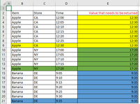
I've got a table with 4 columns(B~D), Item, Store, and Time.

In Column E, I want to write a function that looks up the value from "Item" and "Store", then returns the value of "Time" of the last row where both "Item" and "Store" values are matched.

So for example, E3~E9 will have the value of 12:30 since that is the last row of "Apple" and "CA".

I apologize for the clumsy explanation, please see the attached image for your reference.

Any help will be greatly appreciated.

Thanks
 

Attachments

  • 222.png
    222.png
    24.6 KB · Views: 19

Excel Facts

Excel motto
Not everything I do at work revolves around Excel. Only the fun parts.
you are showing the max(time) did you mean last row or max time - was not sure if just a coincidence it was maximum time and also the last row
 
Upvote 0
you are showing the max(time) did you mean last row or max time - was not sure if just a coincidence it was maximum time and also the last row
Yes, it is the maximum(latest) time.
 
Upvote 0
are you still using 2016 version ,
otherwise a MAXIFS() would work - available from 2019 version
=MAXIFS($D$3:$D$21,$B$3:$B$21,B3,$C$3:$C$21,C3)

Aggregate - added in excel 2010 , so should work in 2016 version
=AGGREGATE(14,6,$D$3:$D$21/(($B$3:$B$21=B3)*($C$3:$C$21=C3)),1)

MAX(IF
=MAX(IF(($B$3:$B$21=B3)*($C$3:$C$21=C3),$D$3:$D$21))

Note i have added a value that is the max time - BUT NOT the last row

Book7
ABCDEFG
1
2MAXIFS()AGGREGATE()MAX(IF(
3AppleCA12:0012:3012:3012:30
4AppleCA12:0512:3012:3012:30
5AppleCA12:1012:3012:3012:30
6AppleCA12:1512:3012:3012:30
7AppleCA12:2012:3012:3012:30
8AppleCA12:2512:3012:3012:30
9AppleCA12:3012:3012:3012:30
10AppleNY17:0017:2017:2017:20
11AppleNY17:0517:2017:2017:20
12AppleNY17:1017:2017:2017:20
13AppleNY17:1517:2017:2017:20
14AppleNY17:2017:2017:2017:20
15BananaDE9:0518:0018:0018:00
16BananaDE9:1018:0018:0018:00
17BananaDE9:1518:0018:0018:00
18BananaDE9:2018:0018:0018:00
19BananaDE18:0018:0018:0018:00
20BananaDE9:3018:0018:0018:00
21BananaDE9:3518:0018:0018:00
Sheet1
Cell Formulas
RangeFormula
E3:E21E3=MAXIFS($D$3:$D$21,$B$3:$B$21,B3,$C$3:$C$21,C3)
F3:F21F3=AGGREGATE(14,6,$D$3:$D$21/(($B$3:$B$21=B3)*($C$3:$C$21=C3)),1)
G3:G21G3=MAX(IF(($B$3:$B$21=B3)*($C$3:$C$21=C3),$D$3:$D$21))
 
Upvote 0

Forum statistics

Threads
1,225,738
Messages
6,186,728
Members
453,368
Latest member
positivemind

We've detected that you are using an adblocker.

We have a great community of people providing Excel help here, but the hosting costs are enormous. You can help keep this site running by allowing ads on MrExcel.com.
Allow Ads at MrExcel

Which adblocker are you using?

Disable AdBlock

Follow these easy steps to disable AdBlock

1)Click on the icon in the browser’s toolbar.
2)Click on the icon in the browser’s toolbar.
2)Click on the "Pause on this site" option.
Go back

Disable AdBlock Plus

Follow these easy steps to disable AdBlock Plus

1)Click on the icon in the browser’s toolbar.
2)Click on the toggle to disable it for "mrexcel.com".
Go back

Disable uBlock Origin

Follow these easy steps to disable uBlock Origin

1)Click on the icon in the browser’s toolbar.
2)Click on the "Power" button.
3)Click on the "Refresh" button.
Go back

Disable uBlock

Follow these easy steps to disable uBlock

1)Click on the icon in the browser’s toolbar.
2)Click on the "Power" button.
3)Click on the "Refresh" button.
Go back
Back
Top