Hi all,
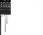
I have a drop down list in cell O2 (color names). Depending on the color I select in the drop down list, column P2:P populates with company names.
Main Purpose -
For each color in the drop down list (O2), I want to make sure that there is only one Company Name attached to it. example for the color Red, Only Microsoft should be shown in column P (no matter how many times). It should not have IBM or any other company name.
1) I would like to create a macro that will automatically go through each color in the drop down list in cell O2.
2) For each color in Cell O2, the macro should check if the corresponding values in column P have different company names.
IF there is only one company name in the column P, THEN do nothing and continue on.
IF there is more than one company name in column P THEN, Copy the color name in cell O2 and paste it to cell S2. Continue on with the code until the very end of the drop down list, cell O2. If the code finds more colors that have multiple company names then copy that color and paste it to the next cell in column S, i.e cell S3, S4, S5 etc.
P.S. I am using a formula in column P that extracts values depending on the color selected in the drop down list. In order to keep the column P dynamic the formula uses IFERROR to blank out cells that give me a NUM error (IFERROR, formula, ""). I would like the macro to only look at company names (values) and ignore the blank cells.
This is the code I used to loop through the drop down list. I'm having trouble with the next part and then merging the whole thing together.
Sub LoopThroughDataValidationList()
Dim rng As Range
Dim dataValidationArray As Variant
Dim i As Integer
Dim rows As Integer
Dim d As Object, c As Variant, b As Long, lr As Long
'Set the cell which contains the Data Validation list
Set rng = Sheets("worksheet1").Range("O2")
'Create an array from the Data Validation formula, without creating
'a multi-dimensional array from the range
rows = Range(Replace(rng.Validation.Formula1, "=", "")).rows.Count
ReDim dataValidationArray(1 To rows)
For i = 1 To rows
dataValidationArray(i) = _
Range(Replace(rng.Validation.Formula1, "=", "")).cells(i, 1)
Next i
'Loop through all the values in the Data Validation Array
For i = LBound(dataValidationArray) To UBound(dataValidationArray)
'Change the value in the data validation cell
rng.Value = dataValidationArray(i)
Next i
End Sub
Thank you for your help.


