VBA Find Cell from Date listed, in Columns, Return cell to highlight in color

[lachelleb]

Afternoon,

I'm pretty new to using VBA and I fear I may have bitten off more than I can chew or have been a bit more overachieving with the task that I'm trying to do. I'm sure that it is something that can be done.
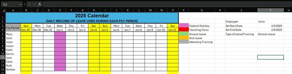
Ultimately, what I'm trying to do is this. This is a calendar for the entire pay year, It has multiple rows for each employee for each pay period (x 26 sections) that include days of week and numbered dates.

At the top in cells T2, an employee would select their name, put in the the start of the leave date (or the date that they would start training) in cell T3, the end of their leave date (or end of training) in cell T4, and the type of leave/training in cell T5.

The code would then search the rows 4,17, 30, 43, 56, 69, 82, 95, 108, 121, 134, 147, 160, 173, 186, 199, 212, 225, 238, 251, 264, 277, 290, 303, 316, 329, 342 for the first date in T3, Then search for the name of the employee in column A, highlight cell where the row and column meet, with the color that matches the training next to the training/leave in column P, then look for the end date in cell T4, and highlight every cell between those rows.

For instance, in the screen shot attached, It would find The date Jan 3, and employee Josie, highlight cell G7, in the Green color, then every offset cell until I7 (which is the end date in cell T4) in the same color.

Then it would save the workbook and clear the entries for the next employee to put their information in.
Maybe perhaps I need to do prompt message boxes. (which I know how to do).

But I can't get it to find the dates. I had some code that was able to search for dates through the rows, but it kept returning no date found.

Here is the code I had found and was testing:

Sub Find_Date()

Dim rng1 As Range
Dim dateStr As String
Dim dateToFind As Date
Dim foundDate As Range

'Get date as string value
dateStr = InputBox("Enter the date to be found")

'Convert string value to date format
dateToFind = DateValue(dateStr)

'Edit Sheet1 to your worksheet name
Set rng1 = Sheets("2025").Range(Cells(1, 1), _
Cells(Rows.Count, 4).End(xlUp))

Set foundDate = rng1.Find(what:=dateToFind, _
LookIn:=xlFormulas, _
LookAt:=xlPart, _
SearchOrder:=xlByRows, _
SearchDirection:=xlNext, _
MatchCase:=False, _
SearchFormat:=False)

If Not foundDate Is Nothing Then
foundDate.Select
Else
MsgBox dateStr & " not found"
End If

End Sub

Any ideas to help me not look like I'm in over my head, or should I just leave it as a workbook and make everyone search for their dates manually and color-code things on their own.

Thanks.

 

[mumps]

It is hard to work with picture. It would be easier to help if you could use the XL2BB add-in (icon in the menu) to attach a screenshot (not a picture) of your sheet. Alternately, you could upload a copy of your file to a free site such as www.box.com or www.dropbox.com. Once you do that, mark it for 'Sharing' and you will be given a link to the file that you can post here. Explain in detail what you want to do referring to specific cells, rows, columns and sheets using a few examples from your data (de-sensitized if necessary).

 

[lachelleb]

It is hard to work with picture. It would be easier to help if you could use the XL2BB add-in (icon in the menu) to attach a screenshot (not a picture) of your sheet. Alternately, you could upload a copy of your file to a free site such as www.box.com or www.dropbox.com. Once you do that, mark it for 'Sharing' and you will be given a link to the file that you can post here. Explain in detail what you want to do referring to specific cells, rows, columns and sheets using a few examples from your data (de-sensitized if necessary).

Here is the drop box link: Dropbox

I think I explained everything I wanted to do in my original post.

At the top in cells T2, an employee would select their name, put in the start of the leave date (or the date that they would start training) in cell T3, the end of their leave date (or end of training) in cell T4, and the type of leave/training in cell T5.

The code would then search the rows 4,17, 30, 43, 56, 69, 82, 95, 108, 121, 134, 147, 160, 173, 186, 199, 212, 225, 238, 251, 264, 277, 290, 303, 316, 329, 342 for the first date in T3, Then search for the name of the employee in column A, highlight cell where the row and column meet, with the color that matches the training next to the training/leave in column P, then look for the end date in cell T4, and highlight every cell between those rows.

For instance, in the screen shot attached, It would find The date Jan 3, and employee Josie, highlight cell G7, in the Green color, then every offset cell until I7 (which is the end date in cell T4) in the same color.

Then it would save the workbook and clear the entries for the next employee to put their information in.

I couldn't get the mini-sheet thing to work on my personal computer, so i know it won't work on my work computer as we aren't allowed to install stuff on there.

 

[Alex Blakenburg]

Using Find with dates is particularly tricky and Excel Tips covered that just this week.

Searching for Dates

If you use a worksheet that contains dates, you might want to search for those dates at some point. This isn't as simple as it may first appear. This tip discusses all the ins and outs of searching for a date in Excel.

excelribbon.tips.net

You have a couple of errors before that though.
• You are using column 4 ("D") to get the Last Row but only Column A is reliably populated to the bottom row.
• You are setting rng1 to only go out to Column D but your search range needs to go out to Column O
• In setting the range BOTH Range AND Cells need to reference the Sheet

For the dates search
• The dates are being generated by a formula so you need to use xlValues (not xlFormulas)
• xlValues is heavily dependent on matching the date format using the displayed format - I have assumed the date is consistently using the same format and that B4 is representative of that format.

See if this works for you:
(perhaps @mumps has another way)

Sub Find_Date()

Dim rng1 As Range
Dim LastRow As Long
Dim dateStr As String
Dim dateToFind As Date
Dim foundDate As Range
Dim firstDate As Range

'Get date as string value
dateStr = InputBox("Enter the date to be found")

'Convert string value to date format
dateToFind = DateValue(dateStr)

'Edit Sheet1 to your worksheet name
With Sheets("2025")
    LastRow = .Range("A" & Rows.Count).End(xlUp).Row
    Set rng1 = .Range(.Cells(1, "A"), .Cells(LastRow, "O"))
    Set firstDate = .Range("B4")                        ' Assume all dates will be using this format
End With

Set foundDate = rng1.Find(what:=Format(dateToFind, firstDate.NumberFormat), _
                LookIn:=xlValues, _
                LookAt:=xlWhole, _
                SearchOrder:=xlByRows, _
                SearchDirection:=xlNext, _
                MatchCase:=False, _
                SearchFormat:=False)

If Not foundDate Is Nothing Then
    foundDate.Select
Else
    MsgBox dateStr & " not found"
End If

End Sub

 

[mumps]

@Alex Blakenburg
Thank you for that Alex. I always have trouble finding a date that is the result of a formula. I will try to use you suggestion to find a solution.

 

[mumps]

Copy and paste this macro into the worksheet code module. Do the following: right click the tab name for your "2025" sheet and click 'View Code'. Paste the macro into the empty code window that opens up. Close the code window to return to your sheet. First enter the employee name, start date and end date and lastly select the leave type in T5. The range will be automatically highlighted. It is very important that you select leave type after entering the other data above because the macro is triggered when you select leave type.

Private Sub Worksheet_Change(ByVal Target As Range)
    If Target.CountLarge > 1 Then Exit Sub
    If Intersect(Target, Range("T5")) Is Nothing Then Exit Sub
    Application.ScreenUpdating = False
    Dim strdate As String, dateToFind1 As Date, dateToFind2 As Date, sDate As String, rLeave As Range, x As Long
    Dim lRow As Long, foundDate1 As Range, foundDate2 As Range, DateFormatCell As Range, rName As Range, rColor As Range
    lRow = Cells.Find("*", SearchOrder:=xlByRows, SearchDirection:=xlPrevious).Row
    sDate = Range("T3")
    eDate = Range("T4")
    dateToFind1 = DateValue(sDate)
    dateToFind2 = DateValue(eDate)
    Set DateFormatCell = Range("B4")
    Set foundDate1 = Range("B4:O" & lRow).Find(what:=Format(dateToFind1, DateFormatCell.NumberFormat), LookIn:=xlValues)
    Set foundDate2 = Range("B4:O" & lRow).Find(what:=Format(dateToFind2, DateFormatCell.NumberFormat), LookIn:=xlValues)
    Set rName = Range("A" & foundDate1.Row & ":A" & lRow).Find(Target.Offset(-3).Value, LookIn:=xlValues, lookat:=xlWhole)
    If Not rName Is Nothing Then
        x = Range("Q3:Q15").SpecialCells(xlCellTypeBlanks).Row
        Set rLeave = Range("Q3:Q" & x).Find(Target.Value, LookIn:=xlValues, lookat:=xlWhole)
        Range(Cells(rName.Row, foundDate1.Column), Cells(rName.Row, foundDate2.Column)).Interior.ColorIndex = rLeave.Offset(, -1).Interior.ColorIndex
    End If
    Application.ScreenUpdating = True
End Sub

 

[lachelleb]

Copy and paste this macro into the worksheet code module. Do the following: right click the tab name for your "2025" sheet and click 'View Code'. Paste the macro into the empty code window that opens up. Close the code window to return to your sheet. First enter the employee name, start date and end date and lastly select the leave type in T5. The range will be automatically highlighted. It is very important that you select leave type after entering the other data above because the macro is triggered when you select leave type.

Private Sub Worksheet_Change(ByVal Target As Range)
    If Target.CountLarge > 1 Then Exit Sub
    If Intersect(Target, Range("T5")) Is Nothing Then Exit Sub
    Application.ScreenUpdating = False
    Dim strdate As String, dateToFind1 As Date, dateToFind2 As Date, sDate As String, rLeave As Range, x As Long
    Dim lRow As Long, foundDate1 As Range, foundDate2 As Range, DateFormatCell As Range, rName As Range, rColor As Range
    lRow = Cells.Find("*", SearchOrder:=xlByRows, SearchDirection:=xlPrevious).Row
    sDate = Range("T3")
    eDate = Range("T4")
    dateToFind1 = DateValue(sDate)
    dateToFind2 = DateValue(eDate)
    Set DateFormatCell = Range("B4")
    Set foundDate1 = Range("B4:O" & lRow).Find(what:=Format(dateToFind1, DateFormatCell.NumberFormat), LookIn:=xlValues)
    Set foundDate2 = Range("B4:O" & lRow).Find(what:=Format(dateToFind2, DateFormatCell.NumberFormat), LookIn:=xlValues)
    Set rName = Range("A" & foundDate1.Row & ":A" & lRow).Find(Target.Offset(-3).Value, LookIn:=xlValues, lookat:=xlWhole)
    If Not rName Is Nothing Then
        x = Range("Q3:Q15").SpecialCells(xlCellTypeBlanks).Row
        Set rLeave = Range("Q3:Q" & x).Find(Target.Value, LookIn:=xlValues, lookat:=xlWhole)
        Range(Cells(rName.Row, foundDate1.Column), Cells(rName.Row, foundDate2.Column)).Interior.ColorIndex = rLeave.Offset(, -1).Interior.ColorIndex
    End If
    Application.ScreenUpdating = True
End Sub

This works perfectly. Thanks so much. Going to study what you did tonight.

 

[mumps]

You are very welcome and thanks to Alex for his input.