VBA Code Error Unable to get the Match property of the WorksheetFunction class

[Jiraya_00]

Hi Everyone,

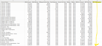
I'm trying to create a macro that will run through a set of column headers and look for a specific header ("CMA - ERP Variance") and calculate a simple formula for all the cells within that column header. However, I'm running into an error with my code as I get the "Run-time error '1004': Unable to get the Match property of the WorksheetFunction class."

Can anyone help me debug this error and let me know what I'm doing wrong? My code is listed below. Thanks for all the help!

Sub Test_MatchReplace()

Dim TestHeader As Long
Dim TestCel As Range, TestCel2 As Range, TestCel3 As Range, TestHeader2 As Range, TestURange As Range
Dim ws As Worksheet

Set ws = ShTest

 With Application
    .StatusBar = "Your macro is running"
    .ScreenUpdating = False
    .DisplayAlerts = False
    .Calculation = xlCalculationManual
    
 End With
 
' To find and replace certain original headers on test data report
 TestHeader = WorksheetFunction.Match("Amount", ShTest.Rows(1), 0)
    Columns(TestHeader).Select
        Selection.Replace What:="Amount", Replacement:="CMA Amount", lookat:=xlWhole _
        , SearchOrder:=xlByRows, MatchCase:=False, SearchFormat:=False, _
        ReplaceFormat:=False, FormulaVersion:=xlReplaceFormula2
        
 TestHeader = WorksheetFunction.Match("Balance", ShTest.Rows(1), 0)
    Columns(TestHeader).Select
        Selection.Replace What:="Balance", Replacement:="CMA Balance", lookat:=xlWhole _
            , SearchOrder:=xlByRows, MatchCase:=False, SearchFormat:=False, _
            ReplaceFormat:=False, FormulaVersion:=xlReplaceFormula2
 
' To create a formula for the "CMA - ERP Variance" column
 TestHeader2 = ShTest.Range(Cells(1, 1), Cells(1, ShTest.Cells(1, Columns.Count).End(xlToLeft).Column))
    
    For Each TestCel In TestHeader2
        If TestCel.Value = "CMA - ERP Variance" Then
            For Each TestCel2 In ShTest.Range("M2:M" & Cells(Rows.Count, "M").End(xlUp).Row)
                If Not IsEmpty(TestCel2.Value) Then
                    TestCel2.Offset(, 2).Formula = "=(RC[-2]-RC[-1])"
                Else
                    TestCel2.Offset(, 2).Value = 0
                End If
            Next TestCel2
        End If
    Next TestCel
 
' To highlight any cells within the "CMA - ERP Variance" column that has a value not equal to 0

 With ShTest
    Set TestURange = .UsedRange
    Set TestURange = .Range("A2").Resize(RowSize:=TestURange.Rows.Count - 1, ColumnSize:=TestURange.Columns.Count)
    For Each TestCel3 In TestURange
        If TestCel3.Column = 15 And TestCel3.Value <> 0 Then
            TestCel3.Interior.ColorIndex = 6
        End If
    Next TestCel3
 End With
 
 With Application
    .StatusBar = ""
    .ScreenUpdating = True
    .DisplayAlerts = True
    .Calculation = xlCalculationAutomatic
    .CutCopyMode = False
    
 End With

End Sub

 

[DanteAmor]

Hi and welcome to MrExcel

I suppose the error is in this line and that is because, according to your image, the data "Amount" does not exist in row 1.

TestHeader = WorksheetFunction.Match("Amount", ShTest.Rows(1), 0)

To avoid this error you can use the find method.
The code can be simplified like this:

Sub Test_MatchReplace()
  Dim f As Range, c As Range
  
  Application.ScreenUpdating = False
  
  ' To find and replace certain original headers on test data report
    Set f = ShTest.Range("1:1").Find("Amount", , xlValues, xlWhole, , , False)
    If Not f Is Nothing Then f.Value = "CMA Amount"
    Set f = ShTest.Range("1:1").Find("Balance", , xlValues, xlWhole, , , False)
    If Not f Is Nothing Then f.Value = "CMA Balance"
  
  ' To create a formula for the "CMA - ERP Variance" column and highlight cell not equal to 0
    Set f = ShTest.Range("1:1").Find("CMA - ERP Variance", , xlValues, xlWhole, , , False)
    If Not f Is Nothing Then
      With f.Offset(1).Resize(ShTest.Range("M" & Rows.Count).End(3).Row - 1)
        .Formula = "=M2-N2"
        For Each c In .Cells
          If c.Value <> 0 Then
            c.Interior.ColorIndex = 6
          End If
        Next
      End With
    End If

  Application.ScreenUpdating = True
End Sub

----- --
Let me know the result and I'll get back to you as soon as I can.
Sincerely
Dante Amor
----- --

 

[Peter_SSs]

Welcome to the MrExcel board!

My code is listed below.

Is that really your code?
If it is, it should never get to the error you mention as it will error at the highlighted line below because ShTest has not been set to anything.

Sub Test_MatchReplace()

Dim TestHeader As Long
Dim TestCel As Range, TestCel2 As Range, TestCel3 As Range, TestHeader2 As Range, TestURange As Range
Dim ws As Worksheet

Set ws = ShTest

BTW, this line is also not a valid line

TestHeader2 = ShTest.Range(Cells(1, 1), Cells(1, ShTest.Cells(1, Columns.Count).End(xlToLeft).Column))

Since TestHeader2 is declared as a Range, the line should be ..

Set TestHeader2 = ShTest.Range(Cells(1, 1), Cells(1, ShTest.Cells(1, Columns.Count).End(xlToLeft).Column))

.. and that line would still only work if ShTest (whatever that is) is the ActiveSheet.

As Dante has said, "Amount" is not found in row 1 of your image - but perhaps your image was taken after the code had already been run or part run and "Amount" had already been replaced by "CMA Amount"?

I have not checked the code any further as I think we need your actual code and confirmation of which line causes the error.

It would also be helpful for our testing if you could provide the sample data with XL2BB rather than as an image that we cannot copy from.

 

[Jiraya_00]

Hello Dante & Peter,

Thank you so much for the feedback! You both are absolutely correct as my code was looking for the two column headers ("Amount" and "Balance") that no longer exists because the first couple lines of the code already found and replaced them.

Dante, after plugging in your code, I no longer run into the error message as I guess it doesn't matter if the two original column headers were there or not. If they are there, then they will be replaced; if not, the code simply moves onto the next line, which is fanstastic!

I did have a question regarding this line of code right here:

With TestFind.Offset(1).Resize(ShTest.Range("M" & Rows.Count).End(3).Row - 1)

Why is it "End(3).Row - 1" and not "End(xlUp).Row"? How will the code know to only fill up the column "CMA - ERP Variance" all the way to last cell within the used range/current region and not autofill it all the way to last cell on the worksheet?

 

[Alex Blakenburg]

Regarding your question, End(3) is the equivalent of End(xlUp). Using 3 is regarded as being undocumented and I would suggest that you stick with using xlUp.
Because that line is not using Range(fromCell, toCell) but using Range(fromCell).Resize(no of rows required) the syntax is slightly different since the no of rows required is the Last Row in Column M minus the Heading Row no which happens to be 1.
This would be more generic in case the heading was not on row 1

With TestFind.Offset(1).Resize(ShTest.Range("M" & Rows.Count).End(xlUp).Row - TestFind.Row)

Discussion on using End(3) here:

End(3) for end(xlup)

Hello All: I read somewhere on the board where there were numbers which can be used to replace XLUP, XLDOWN, XLTOLEFT ect. I use the End(3). However, I'd like to know where to find the other numbers. When I search the board for same, I keep getting no matches found. Can someone enlighten me...

www.mrexcel.com

 

[DanteAmor]

Dante, after plugging in your code, I no longer run into the error message as I guess it doesn't matter if the two original column headers were there or not. If they are there, then they will be replaced; if not, the code simply moves onto the next line, which is fanstastic!

Im glad to help you and thanks for your feedback.


Answering your question:

Why is it "End(3).Row - 1" and not "End(xlUp).Row"?

The number 3 is the numeric value for the xlUp parameter:

You can use xlUp or 3:

xlDown = 4​

xlToLeft = 1​

xlToRight = 2​

xlUp = 3​

--------------------
Set f = ShTest.Range("1:1").Find("CMA - ERP Variance", , xlValues, xlWhole, , , False)

When the Find method encounters the "CMA - ERP Variance" header, the result is stored in the 'f' object​

f.Offset(1).Resize(ShTest.Range("M" & Rows.Count).End(3).Row - 1)

So in object 'f' we have the cell where the header "CMA - ERP Variance" is located, with offset(1) we move one cell down.​

So we have to fill the column from the next cell to the header to the last row with data from the column to M, but we have to subtract 1, because the header is in row 1.​

--------------------

Perform the following test, so that you notice that the formulas are one row below the last row with data in column M:

f.Offset(1).Resize(ShTest.Range("M" & Rows.Count).End(3).Row)

I hope it helps you.

 

[Jiraya_00]

Thank you Dante for this thorough explanation! It definitely helps!

On a side note, I would like to know with the current line of code that I have that will highlight any cell with a value other than zero to be yellow (color index 6) within the "Variance" column. If I correct the variance, and the value then becomes zero, is there a way to have the code automatically remove the yellow highlight? In other words, make it interactive somehow without requiring the user to have to manually remove the yellow highlight themselves?

For Each ReconCel2 In .Cells
       If ReconCel2.Value <> 0 Then
                ReconCel2.Interior.ColorIndex = 6
       End If
Next

 

[DanteAmor]

If I correct the variance, and the value then becomes zero, is there a way to have the code automatically remove the yellow highlight? In other words, make it interactive somehow without requiring the user to have to manually remove the yellow highlight themselves?

I show you some options:

OPTION 1:

If you change the values, you can then run the next macro and it will adjust the colors of the entire column:​

Sub Test_MatchReplace()
  Dim f As Range, c As Range
 
  Application.ScreenUpdating = False
 
  ' To find and replace certain original headers on test data report
    Set f = ShTest.Range("1:1").Find("Amount", , xlValues, xlWhole, , , False)
    If Not f Is Nothing Then f.Value = "CMA Amount"
    Set f = ShTest.Range("1:1").Find("Balance", , xlValues, xlWhole, , , False)
    If Not f Is Nothing Then f.Value = "CMA Balance"
 
  ' To create a formula for the "CMA - ERP Variance" column and highlight cell not equal to 0
    Set f = ShTest.Range("1:3").Find("CMA - ERP Variance", , xlValues, xlWhole, , , False)
    If Not f Is Nothing Then
      With f.Offset(1).Resize(ShTest.Range("M" & Rows.Count).End(3).Row - 3)
        .Formula = "=M2-N2"
        For Each c In .Cells
          If c.Value <> 0 Then
            c.Interior.ColorIndex = 6
          Else
            c.Interior.ColorIndex = xlNone
          End If
        Next
      End With
    End If

  Application.ScreenUpdating = True
End Sub

---------------------------------------------
OPTION 2:

Put a conditional format in the O column:​

varios 19oct2024.xlsm
	E	F	G	H	I	J	K	L	M	N	O
1	Ac	CMA Amount	cma b	mil	tot	serv	reb1	reb2	cma i	erp	CMA - ERP Variance
2	Int	1775	0	45	6	0	0	0	1723	1723	0
3	Int	1776	0	46	0	0	0	0	1724	1724	0
4	Int	1777	0	47	6	0	0	0	1725	1725	0
5	Int	1778	0	48	4	0	0	0	1726	1727	-1
6	Int	1779	0	49	4	0	0	0	1727	1727	0
7	Int	1780	0	50	4	0	0	0	1728	1728	0
8	Int	1781	0	51	4	0	0	0	1729	1720	9
9	Int	1782	0	52	4	0	0	0	1730	1730	0
10	Int	1783	0	53	4	0	0	0	1731	1731	0
11	Int	1784	0	54	4	0	0	0	1732	1732	0
12	Berk	1785	0	55	4	0	0	0	1733	1733	0
13	Berk	1786	0	56	4	0	0	0	1734	1734	0
14	Berk	1787	0	57	4	0	0	0	1735	1735	0
15
ShTest

Cell Formulas
Range	Formula
O2:O14	O2	=M2-N2

Cells with Conditional Formatting
Cell	Condition		Cell Format	Stop If True
O2:O1000	Cell Value	<>0	text	NO

And you delete this part of the macro:

        For Each c In .Cells
          If c.Value <> 0 Then
            c.Interior.ColorIndex = 6
          Else
            c.Interior.ColorIndex = xlNone
          End If
        Next

---------------------------------------------
OPTION 3:
If you modify any value in column M or N, automatically execute a code that reviews the values in column O and sets the color as appropriate:
Put the following code in events of your sheet:

Private Sub Worksheet_Change(ByVal Target As Range)
  Dim rng As Range, c As Range, f As Range
 
  Set rng = Intersect(Target, Range("M2:N" & Rows.Count))
  If Not rng Is Nothing Then
    Set f = Range("1:1").Find("CMA - ERP Variance", , xlValues, xlWhole, , , False)
    If Not f Is Nothing Then
      For Each c In rng
        With Cells(c.Row, f.Column)
          If .Value <> 0 Then
            .Interior.ColorIndex = 6
          Else
            .Interior.ColorIndex = xlNone
          End If
        End With
      Next
    End If
  End If
End Sub

Note Sheet Event:

Right click the tab of the sheet you want this to work, select view code and paste the code into the window that opens up.​

And you delete this part of your macro:

        For Each c In .Cells
          If c.Value <> 0 Then
            c.Interior.ColorIndex = 6
          Else
            c.Interior.ColorIndex = xlNone
          End If
        Next

---------------------------------------------

Option 4:
Delete your macro or you don't use it anymore.. No conditional formatting. Put the following code in your sheet events. Every time you modify a value in the M or N column, it will review the difference between the values you entered, that is, if you modify M5 = 100 and N5 = 98, then the macro automatically sets O5 = 2 and will turn it yellow.

Private Sub Worksheet_Change(ByVal Target As Range)
  Dim rng As Range, c As Range, f As Range
 
  Set rng = Intersect(Target, Range("M2:N" & Rows.Count))
  If Not rng Is Nothing Then
    Set f = Range("1:1").Find("CMA - ERP Variance", , xlValues, xlWhole, , , False)
    If Not f Is Nothing Then
      For Each c In rng
        With Cells(c.Row, f.Column)
          .Value = Cells(c.Row, "M").Value - Cells(c.Row, "N").Value
          If .Value <> 0 Then
            .Interior.ColorIndex = 6
          Else
            .Interior.ColorIndex = xlNone
          End If
        End With
      Next
    End If
  End If

Note Sheet Event:

Right click the tab of the sheet you want this to work, select view code and paste the code into the window that opens up.​

To make it work, simply copy all the values in column n and paste them as values in the same column, the macro will update the entire column O.

From then on the macro will work for one change or for several changes in columns M or N.​

I hope some option works for you.

 

[Jiraya_00]

Thank you Dante! These are all such great options! I will explore and see what works best for my scenario. I had no idea there was even such a thing as sheet event until your post!
I'm definitely learning new things everyday, so thank you again for all your help!