V/Hlookup or Index/Match assistance Required?

[godzilla65]

Hi Team,

I am struggling with the following formula, hoping someone can steer me towards a solution.

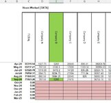
In the Workbook I have a Worksheet Called “Hours Data”, in column B5:B500 I have Dates which are essentially the Months Jan-2012 up to Dec-2024, In row C4:T4, I have a list of companies eg Company A, Company B etc, and for each month we place the total work ours for the month against each company in corresponding cell – This is the source data.

I have another worksheet Company-Stats where I am failing to come up with a formula that I can get working as follows:

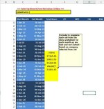
In Cell C3 I have a listbox that has all the Company names, Column C6:C500 is the start of the Month Date eg 01/09/2024, Colum D6:D500 I have the End of Month date eg 30/09/2024, and in column E is where I am failing in my formula.

The formula sounds simple, but I am running into a blank wall, I just wish to select the company form Cell 3, and for every month it populates the hours if the date falls within the start and end dates, for that specific company selected from the data list “Hours Data”

Start Date | End Date | Total Work Hours

01/07/24 31/07/24 36,1234

01/08/24 31/08/24 45,527

01/09/204 30/09/24 25,122

Any help on a formula appreciated!!

Cheers Eric

 

[etaf]

how are the dates formatted in the data sheet - only showing month and year
is that the 1st of the month formatted
OR text

if the date in the data sheet are all 1st month
and the results are all for complete months and start is always 1st month
then a grid lookup should work

what version of excel

i'll mock up and use the grid lookup
EDIT using a grid lookup

does assume the dates are in the correct format


=INDEX(Sheet1!$D$3:$F$5,MATCH(Sheet2!A4,Sheet1!$C$3:$C$5,0),MATCH(Sheet2!$A$1,Sheet1!$D$1:$F$1,0))

Book3
	A	B	C	D	E	F
1				company 1	company 2	company 3
2
3			1-Aug-24	10	100	1100
4			1-Sep-24	11	110	1200
5			1-Oct-24	12	120	1300
6
Sheet1

Cells with Data Validation
Cell	Allow	Criteria
A1	Time	between 00:00:00 and 23:59:00

Book3
	A	B	C
1	company 1
2
3
4	8/1/24	8/31/24	10
5	9/1/24	9/30/24	11
6	10/1/24	10/31/24	12
Sheet2

Cell Formulas
Range	Formula
B4:B6	B4	=EOMONTH(A4,0)
C4:C6	C4	=INDEX(Sheet1!$D$3:$F$5,MATCH(Sheet2!A4,Sheet1!$C$3:$C$5,0),MATCH(Sheet2!$A$1,Sheet1!$D$1:$F$1,0))

 

[godzilla65]

Howdy etaf,

Yes, the dates in the data sheet are all the 1st of the month and formatted, and running on 365 - Microsoft® Excel® for Microsoft 365 MSO (Version 2408 Build 16.0.17928.20114) 64-bit

That would be appreciated as I am stumped.

Cheers Eric

 

[kvsrinivasamurthy]

Try,. In E7 of Sheet2, copied to full column.

=IFERROR(INDEX(Sheet1!$D$3:$K$1000,MATCH($C7,Sheet1!$A$3:$A$1000,0),MATCH($C$4,$D$2:$K$2,0)),"")

 

[etaf]

then the formula I posted modified to match your sheet names and ranges should work OK

Also

kvsrinivasamurthy​

looks the same sort of thing, BUT if it cannot find a match you get an blank cell rather than an error message

it would be worth putting the 365 version in you profile
helps with solutions - as loads of different functions and newer functions in the later version

 

[etaf]

as you are using 365 version then you could use xlookup
=XLOOKUP(A4,Sheet1!$C$3:$C$5,XLOOKUP($A$1,Sheet1!$D$1:$F$1,Sheet1!$D$3:$F$5))

then with an error handling, you can show which element is not being found , also i think it maybe faster performance wise (2 functions v 3 in basic formula0 - but probably not noticeable

=IFERROR(XLOOKUP(A4,Sheet1!$C$3:$C$5,XLOOKUP($A$1,Sheet1!$D$1:$F$1,Sheet1!$D$3:$F$5),"Date Not found"),"Company Not found")

 

[godzilla65]

as you are using 365 version then you could use xlookup
=XLOOKUP(A4,Sheet1!$C$3:$C$5,XLOOKUP($A$1,Sheet1!$D$1:$F$1,Sheet1!$D$3:$F$5))

then with an error handling, you can show which element is not being found , also i think it maybe faster performance wise (2 functions v 3 in basic formula0 - but probably not noticeable

=IFERROR(XLOOKUP(A4,Sheet1!$C$3:$C$5,XLOOKUP($A$1,Sheet1!$D$1:$F$1,Sheet1!$D$3:$F$5),"Date Not found"),"Company Not found")

Thanks heaps - been awhile since I posted, prior to 365 that is for sure, let me process the formula's and revert if I am having any issues - thanks all.

 

[etaf]

delete - duplicated post