Using COUNTIFS with INDIRECT trying to use multiple criteria...Not working.

[iQuikDraw]

Hello,

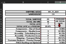
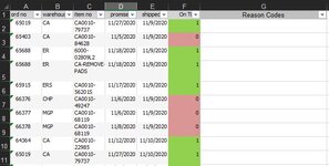
So, I am using the following COUNTIFS formula with INDIRECT to populate the small table (on the left of my dashboard) by looking up which worksheet (Shipping Week) is selected in C5 along with which warehouse is selected in C6 (Column B in the table on the selected worksheet (2nd uploaded imageCapture1.jpg)) as an example of a partial sheet, showing both below…I use this formula to count the number of times the column for “On Time” shipments (Column F) is “0” for late. I do almost the same formula to find the number of times the shipments were “On Time” by replacing the “1” in the formula with a “0”. I then add them together to get the total number of shipments (Rows) in the small table I have on the charts dashboard (uploaded image "Capture.jpg". )

=COUNTIFS(INDIRECT(C5 & "!F:F"),1,INDIRECT(C5 & "!B:B"),C6)

=COUNTIFS(INDIRECT(C5 & "!F:F"),0,INDIRECT(C5 & "!B:B"),C6)

This part works fine...

Column G on the selected worksheet is a (Data Vaildation) list of the reason codes, built directly from the list in the small dashboard table (B8:B11). The numbers generated here are charted to the right of the small dashboard table. For that, I….was…using (For the example of C13):

=COUNTIF(INDIRECT("'"&C5&"'!G:G"),"Components - Quality Issue")

To specifically count the number of times this "Reason Code" occurred in the late shipments...

However, this formula is omitting the reference to the second drop down list in C6, so the charts are being populated only based on the “OnTime” reference entry, not filtering the data by way of the selected warehouse, so the charts always show only the complete totals for the whole worksheet selected. I wish to replace this formula with something similar to:

=COUNTIFS(INDIRECT(C5 & "!F:F"),1,INDIRECT(C5 & "!B:B"),C6,INDIRECT(C6 & "!G:G"),"Components - Quality Issue")

# of times the shipments were late on the given worksheet - Filtered by the selected warehouse in C6 (Column B on the worksheet.), - and again filtered, to only show if the reason code in column G of the worksheet matches the text at the end and the B cell on the dashboard data table.

This formula keeps failing for too many arguments and I can’t seem to get the syntax to work.

I need the two drop down references AND the match to the reason code to all COMBINE for the chart to populate correctly every time I change worksheets in the first drop down list and I change the warehouse in the 2nd drop down list.

I appreciate any help anyone can provide. I'm driving my self nuts changing the syntax many times trying to get better results but I just keep getting errors....

 

[Fluff]

Shouldn't that be C5 in the Indirect function for col G?

 

[iQuikDraw]

Trying that...

 

[iQuikDraw]

I did that and no errors but that brings me back to something not counting right when I can look at the actual worksheet and see that there are 7 entries for that specific "Reason code" and it returns "0". Then I modified the formula to this:

=COUNTIFS(INDIRECT(C5 & "!F:F"),1,INDIRECT(C5 & "!B:B"),C6,INDIRECT(C5 & "!G:G"),B13)

And it still shows "0" as a result. Should be 7

 

[Fluff]

If this formula is giving the correct result

=COUNTIFS(INDIRECT(C5 & "!F:F"),1,INDIRECT(C5 & "!B:B"),C6)

That suggests that either col G doesn't exactly match B13, or there are no rows that meet all three criteria.

 

[iQuikDraw]

This worked...I added the extra Indirect reference back to the list of Reasons on the main page and changed the "1" for true to the first argument to a "0" for false, or, not on time:

=COUNTIFS(INDIRECT(C5 & "!F:F"),0,INDIRECT(C5 & "!B:B"),C6,INDIRECT(C5 & "!G:G"),B13)

 

[Fluff]

Glad you sorted it & thanks for the feedback.