Unique & Filter from multiple tables into a single list

[K1600]

I am curently using

=UNIQUE(FILTER(Table_Std[Course Code],(C2=Table_Std[Start Date])*(Table_Std[Course Cancelled]=""),""))

to return a list of a particular course type planned for a particular date (which is in cell C2), and where the 'Course Cancelled' column is blank i.e. the course has not been cancelled. I use this formula for each course type we run in a single column (column C) over a 171 rows (C150-C321) as there are around 60 possible courses plus the room for the spill.

As we won't have every course running at the same time, to make it easier to read and just see a list of all courses running on the specific day, I am then using

=UNIQUE(FILTER(C150:C321,C150:C321<>""))

to return a single list ignoring all the blank rows.

Is if possible to have a single formula which looks to each of my course tables to check the date and the cancelled column, and then just return a single list rather than me having to have a load of unnecessary rows? I am aware it will be quite a big formula as there are around 60 tables as there is one for each course type, but it will be worth my effort in the long run.

Hope this makes sense.

Thanks in advance.

 

[Cubist]

It would be helpful if you post a sample of your data set, preferably using XL2BB, demonstrating what you're hoping to accomplish.

 

[K1600]

It would be helpful if you post a sample of your data set, preferably using XL2BB, demonstrating what you're hoping to accomplish.

Unfortuanately my work computer won't let me us the XL2BB. I could upload a file but this would take some time as I would need to rebuild it in a new document as I am currently working on a live file and it contains lots of personal data.

 

[Kaper]

How about writing in C1 name table
Table_Std
and then use:

=UNIQUE(FILTER(INDIRECT(C1&"[Course Code]"),($C2=INDIRECT(C1&"[Start Date]"))*(INDIRECT(C1&"[Cancelled]")=""),""))

then you can list all table names in D1, E1, ... and
copy the formula right
and there will be lists for each course types?


Few side comments

- would be nice if to know excel version you are using (next steps can depend on it). You can do it in https://www.mrexcel.com/board/account/
- I also opt for shown sample data set (shorter tables, just 2-3 tables, no personal info) to understand layout (may be tables are stacked vertically? or horizontally with constant width and constant inter-table columns count
- are VBA elements OK in solution?
- Is PQ (Power Query = Get and Transform Data) solution an option - seems it may be the easiest one

 

[Kaper]

PS. As for Power Query I did a sample:
1) in empty workbook I placed a one-row table with date (header in C1 and date in C2 as original. Loaded this table into PQ: Data->Get and transform -> From table-> Load To = Create connection only
2) Data->Get and transform -> From File -> your data file and select multiple item, then check all tables -> Load To = Create connection only
3) Data->Get and transform -> Combine Queries->Append (all but the table with date)
4) In PQ editor Merge Queries The Append one and Date one using Start Date and "C2" date fields, filter on empty cancelled, delete unneded columns, unique (and sort if needed) and finally load to selected cell in a worksheet.

And that's it. The m-code for 3 and 4 steps (case of 2 input tables) looks like:

let
    Source = Table.Combine({Table_Std, Table_NonS}),
    #"Merged Queries" = Table.NestedJoin(Source, {"Start Date"}, DateTbl, {"Date"}, "DateTbl", JoinKind.RightOuter),
    #"Filtered Rows" = Table.SelectRows(#"Merged Queries", each ([Cancelled] = null)),
    #"Removed Other Columns" = Table.SelectColumns(#"Filtered Rows",{"Course Code"}),
    #"Removed Duplicates" = Table.Distinct(#"Removed Other Columns"),
    #"Sorted Rows" = Table.Sort(#"Removed Duplicates",{{"Course Code", Order.Ascending}})
in
    #"Sorted Rows"

The solution was fully clicked-out, nothing coded manually. See screenshol - lest source file, right PQ file

 

[K1600]

How about writing in C1 name table
Table_Std
and then use:

=UNIQUE(FILTER(INDIRECT(C1&"[Course Code]"),($C2=INDIRECT(C1&"[Start Date]"))*(INDIRECT(C1&"[Cancelled]")=""),""))

then you can list all table names in D1, E1, ... and
copy the formula right
and there will be lists for each course types?


Few side comments

- would be nice if to know excel version you are using (next steps can depend on it). You can do it in https://www.mrexcel.com/board/account/
- I also opt for shown sample data set (shorter tables, just 2-3 tables, no personal info) to understand layout (may be tables are stacked vertically? or horizontally with constant width and constant inter-table columns count
- are VBA elements OK in solution?
- Is PQ (Power Query = Get and Transform Data) solution an option - seems it may be the easiest one

Thanks for your response.

Firstly, thanks for the info re the profile update, I have just updated that but for info I am using M365.

I thought that your Power Query suggestion could have been the way forward but thinking about it, (I'm reasonalby new to PQ) I am thinking it will make it run too slowly as if I'm not mistaken, I would need a different query for each day as there will be a column for each day of the year (or at the very least, each working day).

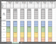
I appreciate my request was a bit complicated so I have created a baisc version but then realised I cannot upload it so I have done some screenshots to hopefuly explain it a bit more and I have outlined the detail below.

The current formula's in the screenshots are:
In the 'Main Sheet'
1. In row 10

=UNIQUE(FILTER(B23:B46,B23:B46<>""))

2. In row 23

=UNIQUE(FILTER(Table_AAA[Course Code],(B2=Table_AAA[Start Date])*(Table_AAA[Course Cancelled]=""),""))

3. In row 29

=UNIQUE(FILTER(Table_BBB[Course Code],(B2=Table_BBB[Start Date])*(Table_BBB[Course Cancelled]=""),""))

4. In row 35

=UNIQUE(FILTER(Table_CCC[Course Code],(B2=Table_CCC[Start Date])*(Table_CCC[Course Cancelled]=""),""))

5. In row 41 (just off screenshot)

=UNIQUE(FILTER(Table_DDD[Course Code],(B2=Table_DDD[Start Date])*(Table_DDD[Course Cancelled]=""),""))

The tables on the 'Courses' tab are named 'Table_AAA', 'Table_BBB', 'Table_CCC' and 'Table_DDD'.

In essence what I am trying to achieve is to have the list of courses that are running that day, populated in the grey cells as they are in rows 10-20 in screenshot, but without the need to have them initially listed in each of the course areas below as they are on the screenshot. I would then do away completly with row 22 onwards. As I said previously, there are many courses but I have only included 4 here.

Hopefully this explains it a bit more.

Thanks in advance.

 

[Cubist]

Is there a reason for having separate tables? It'd be much more efficient if it's just one table.

 

[K1600]

Is there a reason for having separate tables? It'd be much more efficient if it's just one table.

I take it you mean for the courses. If so, the trainers will look at which course they are running in the top section of the 'Main Sheet' sheet (I didn't fill that bit in on the screenshots) and they will then go to the relevent course table to find out who their students are. So if they are running course 21-AAA which would be the 21st instance of course AAA, they would just go to the AAA table and scroll down to 21 to see who their students are. As there are so many courses to have them in a single table I think would be too confusing for them.

 

[Kaper]

I'd also opt for a single table.
Moreover the idea of having redundant information about course (repeated for each student) is not "a way to go" from a point of view of anyone with database experience.
But may be we don't have to follow the rules, so focusing on your sample:

if you use INDIRECT in a formula for row 23, in a way similar to (I've nor recreated a sheet, so could make a typo inside)

=UNIQUE(FILTER(INDIRECT("Table_" & $A23 & "[Course Code]"),(B$2=INDIRECT("Table_" & $A23 & "[Start Date]"))*(INDIRECT("Table_" & $A23 & "[Course Cancelled]")=""),""))

then you can directly (without any changes) copy it (the cell with the formula, not formula in a formula bar) in both directions:
- down to rows 29, 35 and so on
and as a whole range of cells with formulas in column B to columns D, F, H, J and so on.

The main assumption here is that the code of a course listed in column A is the same as in table name after Table_ prefix.

Please note usage of mixed relative/absolute addressing in both date B$2 and course code $A23

 

[K1600]

I'd also opt for a single table.
Moreover the idea of having redundant information about course (repeated for each student) is not "a way to go" from a point of view of anyone with database experience.
But may be we don't have to follow the rules, so focusing on your sample:

if you use INDIRECT in a formula for row 23, in a way similar to (I've nor recreated a sheet, so could make a typo inside)

=UNIQUE(FILTER(INDIRECT("Table_" & $A23 & "[Course Code]"),(B$2=INDIRECT("Table_" & $A23 & "[Start Date]"))*(INDIRECT("Table_" & $A23 & "[Course Cancelled]")=""),""))

then you can directly (without any changes) copy it (the cell with the formula, not formula in a formula bar) in both directions:
- down to rows 29, 35 and so on
and as a whole range of cells with formulas in column B to columns D, F, H, J and so on.

The main assumption here is that the code of a course listed in column A is the same as in table name after Table_ prefix.

Please note usage of mixed relative/absolute addressing in both date B$2 and course code $A23

Thanks, my laptop has just died so I'll give that a whirl tomorrow.

I'm not a fan of the repeated data but because of some other bits that the sheet is used for I'm a bit hand tied with what I can tweak.

Thanks again for your help.