So I have a very long column of data - several thousand rows most of which = close to 0. Between every 140 and 170 (not the same gap every time!) rows I have between 9 and 11 data points that I need. If I use a data filter I get the information I need but i have no way to convert that into multiple columns containing those points. I hope that makes sense, please let me know if you have any ideas!
-
If you would like to post, please check out the MrExcel Message Board FAQ and register here. If you forgot your password, you can reset your password.
Turning filtered data into columns
- Thread starter henrycm
- Start date
SanjayGMusafir
Well-known Member
- Joined
- Sep 7, 2018
- Messages
- 1,535
- Office Version
- 2024
- Platform
- Windows
Just update your version of Excel here and in your profile - The solution will depend upon that.So I have a very long column of data - several thousand rows most of which = close to 0. Between every 140 and 170 (not the same gap every time!) rows I have between 9 and 11 data points that I need. If I use a data filter I get the information I need but i have no way to convert that into multiple columns containing those points. I hope that makes sense, please let me know if you have any ideas!
Upvote
0
SanjayGMusafir
Well-known Member
- Joined
- Sep 7, 2018
- Messages
- 1,535
- Office Version
- 2024
- Platform
- Windows
Henry2016!
Excel 2016 has many limitations compared to the latest versions. That's why I was asking for the version.
The only solution, I can think about is -
- If you can sort that list in ascending or descending order - so as to bring all the data you want to convert to columns may come together at one place (I will try to post an example underneath)
- In case you want to order it back you have to create a fixed index prior or sorting so that you can bring that data back in order it was previously.
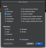
- After sorting in ascending or descending, simply copy (Cmd+C) and paste using (Cmd+Alt+V) keyboard shortcut (THAT's Important).
- A window shall open - There you can choose Paste Values and transpose simultaneously to get the intended result.
- After that if you need you can bring that data back to old sorting using the fixed index you created.
- You can keep or delete that index as per your preference.
| All Records.xlsb | |||||||||||||||
|---|---|---|---|---|---|---|---|---|---|---|---|---|---|---|---|
| A | B | C | D | E | F | G | H | I | J | K | L | M | |||
| 1 | Sorted by Fixed Index | Sorted by Ascending | 2 | 17 | 22 | 46 | 56 | 71 | 94 | ||||||
| 2 | Original List | Fixed Index | Original List | Fixed Index | |||||||||||
| 3 | 56 | 1 | 2 | 14 | |||||||||||
| 4 | 176 | 2 | 17 | 19 | |||||||||||
| 5 | 268 | 3 | 22 | 16 | |||||||||||
| 6 | 46 | 4 | 46 | 4 | |||||||||||
| 7 | 158 | 5 | 56 | 1 | |||||||||||
| 8 | 114 | 6 | 71 | 13 | |||||||||||
| 9 | 264 | 7 | 94 | 15 | |||||||||||
| 10 | 200 | 8 | 104 | 22 | |||||||||||
| 11 | 148 | 9 | 105 | 17 | |||||||||||
| 12 | 235 | 10 | 114 | 6 | |||||||||||
| 13 | 161 | 11 | 130 | 12 | |||||||||||
| 14 | 130 | 12 | 148 | 9 | |||||||||||
| 15 | 71 | 13 | 158 | 5 | |||||||||||
| 16 | 2 | 14 | 161 | 11 | |||||||||||
| 17 | 94 | 15 | 176 | 2 | |||||||||||
| 18 | 22 | 16 | 191 | 23 | |||||||||||
| 19 | 105 | 17 | 200 | 8 | |||||||||||
| 20 | 270 | 18 | 228 | 20 | |||||||||||
| 21 | 17 | 19 | 235 | 10 | |||||||||||
| 22 | 228 | 20 | 238 | 21 | |||||||||||
| 23 | 238 | 21 | 240 | 24 | |||||||||||
| 24 | 104 | 22 | 264 | 7 | |||||||||||
| 25 | 191 | 23 | 268 | 3 | |||||||||||
| 26 | 240 | 24 | 270 | 18 | |||||||||||
Sheet3 | |||||||||||||||
Attachments
Upvote
0
Similar threads
- Solved
- Replies
- 8
- Views
- 222
- Solved
- Replies
- 2
- Views
- 246
- Replies
- 18
- Views
- 320


