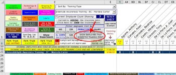
My code looks within a range of cells (employee names which are grouped by columns) and if each target cell does NOT contain an "X", (row 21 in the image below) then it keeps that name visible and hides all other ones that do contain an "X".
note the cells in the dark blue highlighted row with a white x and those with none:

The purpose of this is to provide a count and show which employees missed a specific training event (those with no 'x' missed the selected training event that was previously chosen via one of the two drop-down comboboxes.)
so the current code I have for hiding any cells with 'x's in them and keeping any blank cells unhidden looks like this:
(this code is executed via the command button shown in the next image circled in red w/ a red arrow pointing to it.)
So what I am needing is to change the code to add an 'And' statement that will compare dates from 2 separate cells:
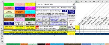
the two cells that I need it to compare are shown below. So row 8 contains the hire date for the employees shown. (I highlighted the one in column R in yellow w red font.)
the cell that each hire date is to be compared to is the date shown in column E in row 21 (again, yellow w red font.)
"If" the hire date for the employee shown is newer than the date shown in column E, then that name (column) is to be hidden along with the cells that do not contain an 'X'. (this is because the specific training date that was chosen happned before that employee was even hired so he (obviously) wouldn't of attended it.)

The dark blue highlighted row (row 23) represents the "For Each" range and is visible where the other non-matching rows are hidden.
The current line of code that shows:
I want to revise so that its saying (in layman terms!):
If the cell value is "" AND, if the date-of-hire value shown is older than the date shown in column E, then keep those cells UNHIDDEN and hide all the others that do not meet those 2 criteria.
So after running the code via the command button you will be left with this (only showing employees that missed the specific training event that happened IF they were hired when the event took place.)

(hope all that makes sense!) Thanks for any help.
note the cells in the dark blue highlighted row with a white x and those with none:

The purpose of this is to provide a count and show which employees missed a specific training event (those with no 'x' missed the selected training event that was previously chosen via one of the two drop-down comboboxes.)
so the current code I have for hiding any cells with 'x's in them and keeping any blank cells unhidden looks like this:
(this code is executed via the command button shown in the next image circled in red w/ a red arrow pointing to it.)
VBA Code:
For Each Cell In Range(Cells(12, 14), Cells(rCol, lCol)).SpecialCells(xlCellTypeVisible)
    If Cell.value = "" Then
        Columns(Cell.Column).Hidden = False
    Else
        Columns(Cell.Column).Hidden = True
    End If
Next
So what I am needing is to change the code to add an 'And' statement that will compare dates from 2 separate cells:
the two cells that I need it to compare are shown below. So row 8 contains the hire date for the employees shown. (I highlighted the one in column R in yellow w red font.)
the cell that each hire date is to be compared to is the date shown in column E in row 21 (again, yellow w red font.)
"If" the hire date for the employee shown is newer than the date shown in column E, then that name (column) is to be hidden along with the cells that do not contain an 'X'. (this is because the specific training date that was chosen happned before that employee was even hired so he (obviously) wouldn't of attended it.)

The dark blue highlighted row (row 23) represents the "For Each" range and is visible where the other non-matching rows are hidden.
The current line of code that shows:
VBA Code:
If Cell.value = "" ThenI want to revise so that its saying (in layman terms!):
If the cell value is "" AND, if the date-of-hire value shown is older than the date shown in column E, then keep those cells UNHIDDEN and hide all the others that do not meet those 2 criteria.
So after running the code via the command button you will be left with this (only showing employees that missed the specific training event that happened IF they were hired when the event took place.)

(hope all that makes sense!) Thanks for any help.


