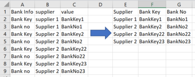
Transpose data to columns

[pjkaphlen]

Hello Excel gurus!

need help in transposing data. Provide is the sample screenshot needed.
Is there a way to do this thru formula or a macro is needed?

Thank you so much!

 

[Fluff]

What version of Excel are you using?

I suggest that you update your Account details (or click your user name at the top right of the forum) so helpers always know what Excel version(s) & platform(s) you are using as the best solution often varies by version. (Don’t forget to scroll down & ‘Save’)

 

[pjkaphlen]

What version of Excel are you using?

I suggest that you update your Account details (or click your user name at the top right of the forum) so helpers always know what Excel version(s) & platform(s) you are using as the best solution often varies by version. (Don’t forget to scroll down & ‘Save’)

Thank you! it has been done now. Been quite some time since I visited my account!

 

[Fluff]

Thanks for that, how about

+Fluff 1.xlsm
	A	B	C	D	E	F	G	H
1						Supplier	Bank Key	Bank No
2	Bank Key	supplier 1	Key1			supplier 1	Key1	No1
3	Bank No	supplier 1	No1			supplier 2	Key2	No2
4	Bank Key	supplier 2	Key2			supplier 2	Key3	No3
5	Bank No	supplier 2	No2			supplier 2	Key4	No4
6	Bank Key	supplier 2	Key3
7	Bank No	supplier 2	No3
8	Bank Key	supplier 2	Key4
9	Bank No	supplier 2	No4
10
Lists

Cell Formulas
Range	Formula
F2:F5	F2	=FILTER(B2:B9,A2:A9=G1)
G2:H5	G2	=INDEX(FILTER($C$2:$C$9,($B$2:$B$9=$F2)*($A$2:$A$9=G$1)),COUNTIFS($F$2:$F2,$F2))
Dynamic array formulas.

 

[pjkaphlen]

That worked like wonders! thank you so much Mod @Fluff!

Thanks for that, how about

+Fluff 1.xlsm
	A	B	C	D	E	F	G	H
1						Supplier	Bank Key	Bank No
2	Bank Key	supplier 1	Key1			supplier 1	Key1	No1
3	Bank No	supplier 1	No1			supplier 2	Key2	No2
4	Bank Key	supplier 2	Key2			supplier 2	Key3	No3
5	Bank No	supplier 2	No2			supplier 2	Key4	No4
6	Bank Key	supplier 2	Key3
7	Bank No	supplier 2	No3
8	Bank Key	supplier 2	Key4
9	Bank No	supplier 2	No4
10
Lists

Cell Formulas
Range	Formula
F2:F5	F2	=FILTER(B2:B9,A2:A9=G1)
G2:H5	G2	=INDEX(FILTER($C$2:$C$9,($B$2:$B$9=$F2)*($A$2:$A$9=G$1)),COUNTIFS($F$2:$F2,$F2))
Dynamic array formulas.

 

[Fluff]

You're welcome & thanks for the feedback.