Toggle Feature on Summary

[volsfan210]

Hi -

Have the below summary that is pulling from a data sheet in excel and this is the current formula.

=SUMPRODUCT(('INITAL ENTRY DATA RAW'!$L$1:$BD$1='PHASE SUMMARY'!D$6)*('INITAL ENTRY DATA RAW'!$L$2:$BD$2='PHASE SUMMARY'!$C7)*'INITAL ENTRY DATA RAW'!$L$4:$BD$1999)

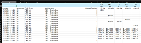
In column D of the initial entry is a code "ABCD" & XYZ". Is there a way to add to add a feature to be able to give me the values based off the Code.

Ideally I would like to be able to filter just the ABCD data or the XYZ data.

Know a Macro is possible just would like to avoid if possible. If you cant avoid a macro any suggestion on an easy macro.

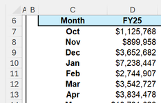
Month	FY25
Oct	$1,125,768​
Nov	$899,958​
Dec	$3,652,682​
Jan	$7,238,447​
Feb	$2,744,907​
Mar	$3,542,727​
Apr	$3,834,478​

 

[myall_blues]

We don't know what's in 'PHASE SUMMARY' or what your data look like, but as an example since you're using 365 you can use a FILTER formula like so:

Book1
	A	B	C	D
1		Code:	ABCD
2			Oct	$1,125,768
3			Nov	$899,958
4			Jan	$7,238,447
5			Mar	$3,542,727
Sheet1

Cell Formulas
Range	Formula
C2:D5	C2	=FILTER('INITIAL ENTRY DATA RAW'!B6:C13,'INITIAL ENTRY DATA RAW'!D6:D13=C1)
Dynamic array formulas.

where the input data on 'INITIAL DATA ENTRY RAW' looks like this:

Book1
	B	C	D
6	Month	FY25	Code
7	Oct	$1,125,768	ABCD
8	Nov	$899,958	ABCD
9	Dec	$3,652,682	XYZ
10	Jan	$7,238,447	ABCD
11	Feb	$2,744,907	XYZ
12	Mar	$3,542,727	ABCD
13	Apr	$3,834,478	XYZ
INITIAL ENTRY DATA RAW

 

[volsfan210]

We don't know what's in 'PHASE SUMMARY' or what your data look like, but as an example since you're using 365 you can use a FILTER formula like so:

Book1
	A	B	C	D
1		Code:	ABCD
2			Oct	$1,125,768
3			Nov	$899,958
4			Jan	$7,238,447
5			Mar	$3,542,727
Sheet1

Cell Formulas
Range	Formula
C2:D5	C2	=FILTER('INITIAL ENTRY DATA RAW'!B6:C13,'INITIAL ENTRY DATA RAW'!D6:D13=C1)
Dynamic array formulas.

where the input data on 'INITIAL DATA ENTRY RAW' looks like this:

Book1
	B	C	D
6	Month	FY25	Code
7	Oct	$1,125,768	ABCD
8	Nov	$899,958	ABCD
9	Dec	$3,652,682	XYZ
10	Jan	$7,238,447	ABCD
11	Feb	$2,744,907	XYZ
12	Mar	$3,542,727	ABCD
13	Apr	$3,834,478	XYZ
INITIAL ENTRY DATA RAW

Hi -

I apologize should have given more detail on the data file I'm pulling from. The months are going across the columns where as the code is in the row.

Attached a sample of the raw data im pulling from "Inital Entry"

 

[myall_blues]

I realise you've provided test data here, but I can't understand how your original formula gave the correct answer as it never refers to the values in column C of your test data.

Nevertheless, based on what you have provided (you will need to modify ranges and sheet name references to suit) you can use a formula such as the one shown at B24.

Book1
	A	B	C	D	E	F						L	M	N	O	P	Q
1												FY25	FY25	FY25	FY25	FY25
2												Oct	Nov	Dec	Jan	Feb
3	Activity ID	Department	FY-G	Group	Activity Name							1/10/2024	1/11/2024	1/12/2024	1/01/2025	1/02/2025
4	TEST-SP01-01-10415	PM	FY26	XYZ	TEST							60132.38
5	TEST-SP01-01-10415	PM	FY26	XYZ	TEST
6	TEST-SP01-01-10415	PM	FY26	XYZ	TEST
7	TEST-SP01-01-10415	PM	FY26	XYZ	TEST								54528.03
8	TEST-SP01-01-10415	PM	FY26	XYZ	TEST
9	TEST-SP01-01-10415	PM	FY26	XYZ	TEST										9725.22
10	TEST-SP01-01-10415	PM	FY26	XYZ	TEST								33596.18	48507.67
11	TEST-SP01-01-10415	PM	FY26	XYZ	TEST
12	TEST-SP01-01-10415	PM	FY26	XYZ	TEST											50662.22
13	TEST-SP01-01-10415	PM	FY26	XYZ	TEST
14	TEST-SP01-01-10525	PM	FY25	ABC	TEST							11600.41	39467.85	50814.57	46442.48	50464.07
15	TEST-SP01-01-10525	PM	FY25	ABC	TEST							5126.48	7359.27	4733.87	19330.63	6635.46
16	TEST-SP01-01-10525	PM	FY25	YYY	TEST							31529.38	42686.71	30189.06	52810.34	9728.72
17	TEST-SP01-01-10525	PM	FY25	ABC	TEST							17122.86	48309.50	25573.63	38651.72	42861.16
18	TEST-SP01-01-10525	PM	FY25	ABC	TEST							35100.59	40981.71	18660.42	27356.08	43991.75
19	TEST-SP01-01-10525	PM	FY25	ABC	TEST							18310.05	59284.26	45390.58	10468.25	3767.33
20	TEST-SP01-01-11030	PM	FY28	XYZ	TEST
21
22
23	Criteria:
24	FY25	Oct	87260.39
25	ABC	Nov	195402.6
26		Dec	145173.1
27		Jan	142249.2
28		Feb	147719.8
29
30
INITAL ENTRY DATA RAW

Cell Formulas
Range	Formula
L1:P1	L1	="FY" & (YEAR(L3)+(MONTH(L3)>=7)-2000)
L2:P2	L2	=TEXT(L3,"mmm")
B24:C68	B24	=IFERROR(LET(_a,VSTACK(L2:BD2,BYCOL(FILTER(FILTER(L4:BD20,(C4:C20=A24)*(D4:D20=A25)),(L1:BD1=A24)),LAMBDA(array,SUM(array)))), TRANSPOSE(IF(_a=0,"",_a))),"")
Dynamic array formulas.