SUMIFS formula on multiple criteria

[Nlambert]

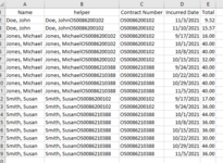
I am trying to find a way to sum a range of values based upon multiple criteria. Primarily I need to sum all of the hours worked from a raw report based on an employee name, contract number, and the month worked into a second worksheet within the same workbook.

I have created "helper" cells to try and make it easier, but any time I try to return a result based upon a SUMIFS formula, the result is always 0. What am I doing wrong?

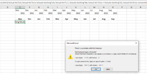
I've attached a sample image as I cannot download on my work PC. Actuals Raw = raw report (with helper added). Actuals Working (where I want the calculations to occur, pulling data from the Raw worksheet)

 

[jasonb75]

Are the month names in the Working sheet proper dates formatted as month, or simply text strings?

You don't need the helper columns, just a valid formula. The basic syntax would be like this, you just need to replace the lower case descriptions with valid references in your Working sheet.

=SUMIFS(RAW!$E:$E,RAW!$A:$A,name,RAW!$C:$C,contract,RAW!$D:$D,">="&start of month, RAW!$D:$D,"<="&end of month)

 

[Nlambert]

Most are, however I am having issues with the formatting of the date columns. I need it specifically to separate 2021 and 2022, however if I try to add a helper column that converts the date of 11/21/21 (for example) to Nov2021, it will force the cell to be a custom format. I haven't found a way around that just yet.

 

[jasonb75]

Delete all of the helpers, they are absolutely useless for what you are doing.

Enter the date as 11/01/21 into what I believe is E5 of the Working sheet (currently shows Nov in bold). In F5, enter the formula =EDATE(E5,1) and drag right as far as O5. Apply a custom format of mmm to these dates.

Then enter this formula into E6 and use it to fill the table.

=SUMIFS(RAW!$E:$E,RAW!$A:$A,$A6,RAW!$C:$C,$B6,RAW!$D:$D,">="E$5, RAW!$D:$D,"<"&EOMONTH($E5,0))

 

[Nlambert]

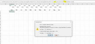
I've gotten the formatting to take, however I get an error when trying to either paste this formula or when i try to type it out. I've ensured that the reference cells are correct, formatting is on point, and the formula makes logical sense stepping through it. Any suggestions?

Note - I have not yet included the $ as I was trying to see if the formula would take first. I also had to remove the " " around the >= and < signs due to it not allowing me to select the reference date cell otherwise.

 

[petertenthije]

Why do you want to do this through formulas? A pivot table can do the same and be quicker at it.

 

[Nlambert]

Why do you want to do this through formulas? A pivot table can do the same and be quicker at it.

There are about 6 tabs on this sheet, and other worksheets reference these same cells and worksheets. These reports come out of our system and I am trying to avoid adding additional pivot tables that have to manually be added every time a new report is ran. My ultimate goal is to be able to paste in the new report and not have to touch it. There is another worksheet after this one that will reference this sheet for final data, once I have determined how to pull it.

 

[Fluff]

I also had to remove the " " around the >= and < signs

You cannot do that, the quotes must be in the formula.

 

[Nlambert]

When I add in the quotes, I get the attached error. Without the quotes I don't get the error, but the sum is always 0.

You cannot do that, the quotes must be in the formula.

 

[Fluff]

You're missing the ampersand before E5

Without the quotes I don't get the error

I very much doubt that.