sumif or sumifs formula which does not sum if one or more of the values is zero.

[JoCil]

Hi, I am new to the forum, but have used several of the great solutions posted here in the past.

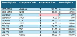
The attached screenshot illustrates my current challenge better than I can describe it, but I'll try :
The first column contains assembled (complete) product codes.
The second column contains the components which goes into the making of the assembled products, and there can be two or more components per assembled product.
The third column looks up each component price from elsewhere.
The last column is a sumif formula which totals each component price for that completed product.

The problem is that if the component price (from elsewhere) is missing (zero), the assembled product price is incorrect, and should rather default to zero.

I mainly work with excel tables hence the current assembled price formula is:
=SUMIFS([ComponentPrice],[AssemblyCode],[@AssemblyCode])

I searched for a solution and there were some that are related, but not quite what I need.
Some solutions suggested using combined IF and COUNTIF functions to identify if zeros appear in the range, but this then cancels ALL the assembled price calculations, even if they are correct.

I also tried the following without success:
=SUMIFS([ComponentPrice],[AssemblyCode],[@AssemblyCode],"<>")
=SUMIFS([ComponentPrice],[AssemblyCode],[@AssemblyCode],">0")

Any suggestions, please?

(PS, the table is just a simplified explanation of the issue so please ignore the fact that the component price is duplicated per each component of an assembled product on the screenshot of the table)

 

[Eric W]

Try:

Book1
	A	B	C	D
1	AssemblyCode	ComponentCode	ComponentPrice	AssemblyPrice
2	A	1	102	132
3	A	2	30	132
4	B	1		0
5	B	2	6	0
6	C	1	200	206
7	C	2	6	206
8	D	1	150	335
9	D	2	51	335
10	D	3	46	335
11	D	4	88	335
Sheet3

Cell Formulas
Range	Formula
D2:D11	D2	=IF(COUNTIFS([AssemblyCode],[@AssemblyCode],[ComponentPrice],">0")=COUNTIF([AssemblyCode],[@AssemblyCode]),SUMIFS([ComponentPrice],[AssemblyCode],[@AssemblyCode]),0)

 

[Peter_SSs]

Welcome to the MrExcel board!
For the future, please consider XL2BB for your sample data so that helpers can easily copy it to test with.

A marginally shorter option that I think should also work for you.

JoCil.xlsm
	A	B	C	D
1	AssemblyCode	ComponentCode	ComponentPrice	AssemblyPrice
2	A	1	$ 102.00	$ 132.00
3	A	2	$ 30.00	$ 132.00
4	B	1	$ -	$ -
5	B	2	$ 6.00	$ -
6	C	1	$ 200.00	$ 206.00
7	C	2	$ 6.00	$ 206.00
8	D	1	$ 150.00	$ 335.00
9	D	2	$ 51.00	$ 335.00
10	D	3	$ 46.00	$ 335.00
11	D	4	$ 88.00	$ 335.00
Sheet1

Cell Formulas
Range	Formula
D2:D11	D2	=SUMIFS([ComponentPrice],[AssemblyCode],[@AssemblyCode])*(MINIFS([ComponentPrice],[AssemblyCode],[@AssemblyCode])>0)

 

[KRice]

Another idea to consider:
EDIT: I should add...this assumes the missing prices are blanks, not 0's....so this may not work for you.

Book2
	A	B	C	D
1	AssemblyCode	ComponentCode	ComponentPrice	AssemblyPrice
2	a	p	1	1
3	b	d	2	2
4	c	q		0
5	c	f	3	0
6	d	r	4	9
7	d	g	5	9
8	e	s	6	30
9	e	t	7	30
10	e	x	8	30
11	e	y	9	30
Sheet3

Cell Formulas
Range	Formula
D2:D11	D2	=LET(a,FILTER([ComponentPrice],[AssemblyCode]=@[AssemblyCode]),IF(XOR(ISBLANK(a)),0,SUM(a)))

Similar version that accounts for 0's:

Book2
	A	B	C	D
1	AssemblyCode	ComponentCode	ComponentPrice	AssemblyPrice
2	A	1	102	132
3	A	2	30	132
4	B	1	0	0
5	B	2	6	0
6	C	1	200	206
7	C	2	6	206
8	D	1	150	335
9	D	2	51	335
10	D	3	46	335
11	D	4	88	335
Sheet4

Cell Formulas
Range	Formula
D2:D11	D2	=LET(a,FILTER([ComponentPrice],[AssemblyCode]=@[AssemblyCode]),IF(XOR(a>0),0,SUM(a)))

 

[Eric W]

Hi Peter, the value in C4 is undoubtably 0, based on the original formatting. And your formula works fine if that's the case. But I noticed that if that cell is empty "" , then your formula fails, which is why I went with the longer version. Probably not an issue though.

KRice, your formula has the opposite issue. If the value is 0, it fails. Moreover, if 2 components are empty (or any even number), then it also fails. But an interesting approach!

 

[KRice]

Thanks,..good point, Eric!...and my 2nd quick edit fails too. Hmmm...

 

[Eric W]

Thanks,..good point, Eric!...and my 2nd quick edit fails too. Hmmm...

Maybe:

Book1
	A	B	C	D
1	AssemblyCode	ComponentCode	ComponentPrice	AssemblyPrice
2	A	1	$ 102.00	132
3	A	2	$ 30.00	132
4	B	1	$ -	0
5	B	2	$ 6.00	0
6	C	1	$ 200.00	206
7	C	2	$ 6.00	206
8	D	1	$ 150.00	0
9	D	2		0
10	D	3	$ 46.00	0
11	D	4		0
Sheet3

Cell Formulas
Range	Formula
D2:D11	D2	=LET(a,FILTER([ComponentPrice],[AssemblyCode]=@[AssemblyCode]),IF(OR(a=0),0,SUM(a)))

 

[KRice]

Eric, yes, that's a good adjustment, and it handles 0's and blanks...and multiple 0's and blanks. Thank you.

 

[Peter_SSs]

Hi Peter, the value in C4 is undoubtably 0, based on the original formatting. And your formula works fine if that's the case. But I noticed that if that cell is empty "" ,

Hi Eric. Apart from the formatting indication, my reading of it was that we were told that it was zero

The problem is that if the component price (from elsewhere) is missing (zero), ..

 

[JoCil]

Try:

Book1
	A	B	C	D
1	AssemblyCode	ComponentCode	ComponentPrice	AssemblyPrice
2	A	1	102	132
3	A	2	30	132
4	B	1		0
5	B	2	6	0
6	C	1	200	206
7	C	2	6	206
8	D	1	150	335
9	D	2	51	335
10	D	3	46	335
11	D	4	88	335
Sheet3

Cell Formulas
Range	Formula
D2:D11	D2	=IF(COUNTIFS([AssemblyCode],[@AssemblyCode],[ComponentPrice],">0")=COUNTIF([AssemblyCode],[@AssemblyCode]),SUMIFS([ComponentPrice],[AssemblyCode],[@AssemblyCode]),0)

Hi Eric,
This does the job, thank you VERY much !