SUMIF but with Calculation First

[Spyderturbo007]

Hopefully someone can help me. I have a printer that spits out data associated with every print job that includes material cost, surface treatment cost, ink volume, etc. Each print job is a different CSV file. I found a way to combine them all using the Data -> Get Data option.
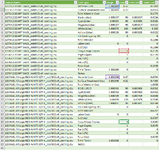
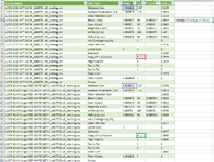
I'm trying to find a way to run a calculation for each print job, but I need it to do a calculation before the summation. I need to take the product of Material Cost Usage and Copy Group Copies and then add them together for each Source.Name.

In the case of these first two it would be =SUM((C2*D14),(C21*D33))

The problem is that there are about 1000 different Source.Name entries in this sheet so doing it manually would be impossible. Ultimately, I'd like to be able to figure out total ink usage as well, but I think if I can get the syntax of one down, I can figure out the others.

Hopefully this makes sense. Thanks so much for the help!

 

[Herakles]

=SUM((C2*D14),(C21*D33))

Where is the cell containing this calulation to be?

Do you have a summary sheet with a single row for each print job?

 

[Spyderturbo007]

My apologies, but my original screenshot was incorrect. I removed part of the file name for privacy reasons and didn't realize that I filled it down as opposed to copying it down so Excel automatically incremented the number. I'm attaching the correct screenshot to this post.

As for the location of the calculation, it doesn't matter to me. Once I get the syntax of the calculation and the correct function, I can manipulate it to look pretty if needed.

Unfortunately, the software creates a single CSV file during the print job for each file.

 

[Herakles]

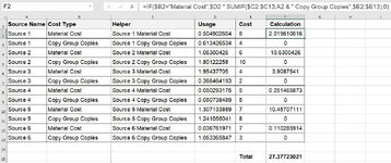
I would create a hidden helper column after the [Cost Type] column.

Concatenate the values in the [Source.Name] and the [Cost Type] columns in this helper column.

Create a new column and use a formula to do the calculation exampled in the image for each [Source.Name] but only
against the [Cost Type] that is 'Material Cost'.

The sum of this column is what you are after.

 

[Spyderturbo007]

@Herakles Thank you for the help! I'm just getting back to this today. Can you help me with the Concatenate part? I am vaguely familiar with that function, but mine ends up as SourceNameCostType stuck together. It looks like yours is separate rows for SourceName and Cost Type.

 

[Sufiyan97]

Are you using CONCATE formula like this?

=CONCAT(A2," ",B2)

 

[Sufiyan97]

Try

Book3
	A	B	C	D	E	F	G	H	I	J	K
1	Source Name	Cost Type	Usage	Cost
2	Source 1	Material Cost	0.302489			Source Name	Material Cost * Copy Group Copies
3	Source 1	Surface	0.302489			Source 1	0.302489		Total	59.71391
4	Source 1	Copy Group Copies		1		Source 2	7.411424
5	Source 2	Material Cost	1.852856			Source 3	10
6	Source 2	Surface	1.852856			Source 4	12
7	Source 2	Copy Group Copies		4		Source 5	14
8	Source 3	Material Cost	5			Source 6	16
9	Source 3	Surface					0
10	Source 3	Copy Group Copies		2
11	Source 4	Material Cost	6
12	Source 4	Surface
13	Source 4	Copy Group Copies		2
14	Source 5	Material Cost	7
15	Source 5	Surface
16	Source 5	Copy Group Copies		2
17	Source 6	Material Cost	8
18	Source 6	Surface
19	Source 6	Copy Group Copies		2
20
Sheet2

Cell Formulas
Range	Formula
G3:G9	G3	=IFERROR(INDEX($C$2:$C$19,MATCH(F3:F9&"Material Cost",$A$2:$A$19&$B$2:$B$19,0))*INDEX($D$2:$D$19,MATCH(F3:F9&"Copy Group Copies",$A$2:$A$19&$B$2:$B$19,0)),0)
J3	J3	=SUM(IFERROR(INDEX($C$2:$C$19,MATCH(F3:F9&"Material Cost",$A$2:$A$19&$B$2:$B$19,0))*INDEX($D$2:$D$19,MATCH(F3:F9&"Copy Group Copies",$A$2:$A$19&$B$2:$B$19,0)),0))
Dynamic array formulas.