Sum values associated with keywords inside cell

[witchcraftz]

I have a spreadsheet in which I need to do something unusual.

The setup:
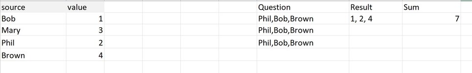
Each cell will contain a list of keywords. Each keyword is worth a specific value (1-4). A cell may contain any number of keywords in any order, however each keyword only repeats once.

Data sheet

source	value
Bob	1
Mary	3
Phil	2
Brown	4

Results sheet

input	value list	value sum
Phil,Bob,Brown	1, 2, 4	7

Part1 :Getting a list that transposes the words in the cell to a list of associated values.

I've done this 2 ways but I feel both are ugly and nonuser friendly, would be great if someone had a better/simpler way to do this.

In the results sheet I expect the value list to return 1, 2, 4 (in any order is fine)

These work but are ugly:

Option1: =TEXTJOIN(", ", TRUE, IF(COUNTIF(results!A2, "*"&data!A2:A5&"*"), data!B2:B5, ""))

Option2: =IF(ISNUMBER(FIND("Bob",results!A2,1))=TRUE,"1, ","")&IF(ISNUMBER(FIND("Mary",results!A2,1))=TRUE,"3, ","")&IF(ISNUMBER(FIND("Phil",results!A2,1))=TRUE,"2, ","")&IF(ISNUMBER(FIND("Brown",results!A2,1))=TRUE,"4, ","")


Part2 : Sum up the associated values for every word in the cell.

I've looked at sumifs and sumproduct but I couldn't get this to work!

The uploaded image shows what the result should be

 

[jasonb75]

These work but are ugly:

I would say that your desired output is far less attractive than your attempt at resolving it. Excel is not meant to work with a list of items in a single cell, if that is what you want then it is simply a case of finding something that works. Option 1 is the best you're going to get for the value list. For the sum you could try

=SUMPRODUCT(--ISNUMBER(SEARCH(Data!A2:A5,A2)),Data!B2:B5)

 

[Peter_SSs]

I suggest that you update your Account details (or click your user name at the top right of the forum) so helpers always know what Excel version(s) & platform(s) you are using as the best solution often varies by version. (Don’t forget to scroll down & ‘Save’)

I assume that you are aware that the formulas are not actually checking for keywords, but key strings so that you may get a sum even if none of the key words are present?

21 11 16.xlsm
	A	B	C	D	E	F
1	Source	Value		Input	Value list	Value Sum
2	Bob	1		Rosemary,Macphillamy,Nabob,Brownlee	1, 2, 3, 4	10
3	Mary	2
4	Phil	3
5	Brown	4
Sample

Cell Formulas
Range	Formula
E2	E2	=TEXTJOIN(", ", TRUE, IF(COUNTIF(D2, "*"&A2:A5&"*"), B2:B5, ""))
F2	F2	=SUMPRODUCT(--ISNUMBER(SEARCH(A2:A5,D2)),B2:B5)

 

[witchcraftz]

Thanks for the help!

In answer to the keystrings, yes, I am aware however it's good of you to let others know if they try to use the same solution.
This data has been sanitized to avoid disclosing important info. In the actual data each one is very unique.