Rearranging data

[excel_beta_345User]

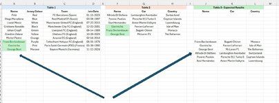
I have two tables as per attached images. Now I want to take data from table 2 and arrange that in table 3 in such order that it matches names as per Column A from table 1. If name matches the cell from Colum A of table 1 A then only it should list all the details in row in table 3. In case if it does not match then it should not be added at all, row should remain blank. It would be great if those non-matched name and their details from table 2 are added at the end of table 3 but if not, I can apply conditional formatting to find out those non matching between table 2 and 3 and cut paste them to move out at the end of table 3, hope that works.

Common factor between table 1 and 3 should be Column with Header "Name". Name in column J should be able to match the same order as of Column A. Can you please help to achieve this?

Sorry that I cannot use XL2BB add-in, unfortunately 0365 policies does not allow that hence had to share image again.

 

[Fluff]

How about

=SORTBY(F3:H8,XMATCH(F3:F8,A3:A12))

 

[excel_beta_345User]

How about

=SORTBY(F3:H8,XMATCH(F3:F8,A3:A12))

yes, it brings the result but does not order it as per A3:A12

 

[Alex Blakenburg]

I'm sure it can be done with less code than this but try:

=LET(orig,F3:H8,
srt,A3:A12,
srtCnt,ROWS(srt),
origCol1,INDEX(orig,0,1),
srtOrder,srtCnt-IFERROR(XMATCH(origCol1,srt,0),-1),
combined,HSTACK(orig,srtOrder),
srtCol,COLUMNS(combined),
DROP(SORTBY(combined,INDEX(combined,0,srtCol)),,-1))

 

[excel_beta_345User]

I'm sure it can be done with less code than this but try:

=LET(orig,F3:H8,
srt,A3:A12,
srtCnt,ROWS(srt),
origCol1,INDEX(orig,0,1),
srtOrder,srtCnt-IFERROR(XMATCH(origCol1,srt,0),-1),
combined,HSTACK(orig,srtOrder),
srtCol,COLUMNS(combined),
DROP(SORTBY(combined,INDEX(combined,0,srtCol)),,-1))

Thank you for the help but unfortunately it is still not fixing the order, after applying this order appears as below. It should be as per sequence from Table 1 Column A

George Best

Garrincha

Franz Beckenbauer

Alfredo Di Stéfano

Ferenc Puskás

Xavi Hernández

 

[Alex Blakenburg]

OK minor adjustment try this:

=LET(orig,F3:H8,
srt,A3:A12,
srtCnt,ROWS(srt),
origCol1,INDEX(orig,0,1),
srtOrder,IFERROR(XMATCH(origCol1,srt,0),srtCnt+1),
combined,HSTACK(orig,srtOrder),
srtCol,COLUMNS(combined),
DROP(SORTBY(combined,INDEX(combined,0,srtCol)),,-1))

 

[Eric W]

How about:

Book1
	A	B	C	D	E	F	G	H	I	J	K	L
1
2	Name	Jersey	Team	Date		Name	Car	Country		Name	Car	Country
3	Pele					Alfredo Di Stefano	G3	H3		Franz Beckenbauer	G7	H7
4	Diego Maradona					Ferenc Puskas	G4	H4		Garrincha	G6	H6
5	Lionel Messi					Xavi Hernandez	G5	H5		George Best	G8	H8
6	Cristiano Ronaldo					Garrincha	G6	H6		Alfredo Di Stefano	G3	H3
7	Johan Cruyff					Franz Beckenbauer	G7	H7		Ferenc Puskas	G4	H4
8	Szinedine Zidane					George Best	G8	H8		Xavi Hernandez	G5	H5
9	Michel Platini
10	Franz Beckenbauer
11	Garrincha
12	George Best
13
Sheet5

Cell Formulas
Range	Formula
J3:L8	J3	=SORTBY(F3:H8,XLOOKUP(F3:F8,A3:A12,ROW(A3:A12),999,0))
Dynamic array formulas.

 

[Cubist]

I fail to see why Fluff's formula didn't work for you.

 

[Alex Blakenburg]

I don't know why I thought I needed to provide an alternative to a straight and simpler SortBy approach . All the above methods produce the same results and I can't reproduce the results in post #5.
Can you post (by copy pasting) the exact formula you are using (please use either Fluff's or Eric's).
If the results deviate from Post #5 show us the results you are getting.

Also an image showing the Row and Column References for both Table1 & Table2.
Ideally add a column to Table2 and do an XMatch to Table1 and check that anything that should be matching is matching.

 

[Peter_SSs]

See if this is what you want.

25 01 23.xlsm
	A	B	C	D	E	F	G	H	I	J	K	L
2	Name	Jersey	Team	Date		Name	Car	Country		Name	Car	Country
3	Pele					Alfredo Di Stefano	G3	H3
4	Diego Maradona					Ferenc Puskas	G4	H4
5	Lionel Messi					Xavi Hernandez	G5	H5		Lionel Messi	G9	H9
6	Cristiano Ronaldo					Garrincha	G6	H6
7	Johan Cruyff					Franz Beckenbauer	G7	H7
8	Szinedine Zidane					George Best	G8	H8
9	Michel Platini					Lionel Messi	G9	H9
10	Franz Beckenbauer									Franz Beckenbauer	G7	H7
11	Garrincha									Garrincha	G6	H6
12	George Best									George Best	G8	H8
13										Alfredo Di Stefano	G3	H3
14										Ferenc Puskas	G4	H4
15										Xavi Hernandez	G5	H5
16
Rearrange

Cell Formulas
Range	Formula
J3:L15	J3	=VSTACK(MAKEARRAY(ROWS(A3:A12),3,LAMBDA(r,c,IFERROR(INDEX(F3:H9,MATCH(INDEX(A3:A12,r),F3:F9,0),c),""))),FILTER(F3:H9,ISNA(MATCH(F3:F9,A3:A12,0))))
Dynamic array formulas.