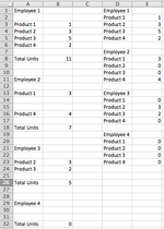
I have a report with information that I want to pull into a table. The report lists names of sales employees, and below that it lists how many units of each product they've sold. If they have not sold a product however, the product name will not appear on the report under the employee's name. For example, if Employee A has sold at least one of each product, all products will populate beneath their name with the quantity sold next to it. If Employee B has sold every product except one, then that one product will not appear on the report. The products are always listed in the same order, and if the first product in the list has not been sold by the employee, the entire row will be missing from the sheet. However, if the employee has only sold the first product on the list and the last product on the list, then there will be entirely blank rows on the sheet for each product the employee did not sell.
-
If you would like to post, please check out the MrExcel Message Board FAQ and register here. If you forgot your password, you can reset your password.
Pulling data from an inconsistent sheet into a consistent table.
- Thread starter Coien
- Start date
Anthony47
Well-known Member
- Joined
- Mar 29, 2006
- Messages
- 3,934
- Office Version
- 365
- 2010
- Platform
- Windows
So lets suppose you have on Sheet1 a report like this:
Now the basic rule is "sh** in - sh** out"
But f you want to dare your fate then go to Sheet2; create in column A the list with the employee name followed by the full list of product (the yellow area in the following XL2BB minisheet), STARTING from Row2 (leave A1 empty)
Now set in B3 the following formula:
Copy down for as many rows are in column A
My output:
| Cartel1 | |||||
|---|---|---|---|---|---|
| A | B | C | |||
| 1 | Inconsistent List | ||||
| 2 | |||||
| 3 | Employee1 | ||||
| 4 | AA | 1 | |||
| 5 | BB | 2 | |||
| 6 | CC | 3 | |||
| 7 | DD | 4 | |||
| 8 | |||||
| 9 | Total Units | 10 | |||
| 10 | |||||
| 11 | |||||
| 12 | |||||
| 13 | Employee2 | ||||
| 14 | |||||
| 15 | BB | 22 | |||
| 16 | CC | 23 | |||
| 17 | |||||
| 18 | |||||
| 19 | Total Units | 45 | |||
| 20 | |||||
| 21 | Employee3 | ||||
| 22 | |||||
| 23 | |||||
| 24 | |||||
| 25 | Total Units | 0 | |||
Sheet1 | |||||
Now the basic rule is "sh** in - sh** out"
But f you want to dare your fate then go to Sheet2; create in column A the list with the employee name followed by the full list of product (the yellow area in the following XL2BB minisheet), STARTING from Row2 (leave A1 empty)
Now set in B3 the following formula:
Excel Formula:
=LET(EMPL,INDIRECT("A"&1+MAX(IF($A$1:A1="",ROW($A$1:A1),""))),myBLKs,MATCH(EMPL,Sheet1!$A$1:$A$100,0),myBLKe,MATCH("Total Units",INDIRECT("Sheet1!A"&myBLKs&":A100"),0),mayBE,IFERROR(VLOOKUP(A3,INDIRECT("Sheet1!A"&myBLKs&":B"&myBLKe+myBLKs),2,0),0),IF(AND(A3<>"",A2<>""),mayBE,""))My output:
| Cartel1 | ||||
|---|---|---|---|---|
| A | B | |||
| 1 | ||||
| 2 | Employee1 | Qty | ||
| 3 | AA | 1 | ||
| 4 | BB | 2 | ||
| 5 | CC | 3 | ||
| 6 | DD | 4 | ||
| 7 | ||||
| 8 | Employee2 | |||
| 9 | AA | 0 | ||
| 10 | BB | 22 | ||
| 11 | CC | 23 | ||
| 12 | DD | 0 | ||
| 13 | ||||
| 14 | Employee3 | |||
| 15 | AA | 0 | ||
| 16 | BB | 0 | ||
| 17 | CC | 0 | ||
| 18 | DD | 0 | ||
| 19 | ||||
| 20 | ||||
Sheet2 | ||||
| Cell Formulas | ||
|---|---|---|
| Range | Formula | |
| B3:B20 | B3 | =LET(EMPL,INDIRECT("A"&1+MAX(IF($A$1:A1="",ROW($A$1:A1),""))),myBLKs,MATCH(EMPL,Sheet1!$A$1:$A$100,0),myBLKe,MATCH("Total Units",INDIRECT("Sheet1!A"&myBLKs&":A100"),0),mayBE,IFERROR(VLOOKUP(A3,INDIRECT("Sheet1!A"&myBLKs&":B"&myBLKe+myBLKs),2,0),0),IF(AND(A3<>"",A2<>""),mayBE,"")) |
Upvote
0
Similar threads
- Question
- Replies
- 1
- Views
- 291
- Replies
- 2
- Views
- 284
- Solved
- Replies
- 2
- Views
- 142
- Replies
- 1
- Views
- 653


