partial text lookup /match in a table and return value with date range and return the month sum value

[Batata]

Hello,

I am wondering if someone could help me with the following because I'm stuck with my formula, and I think it's too complicated for my level.

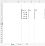
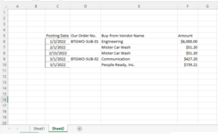
An example below is trying to explain what exactly I want from the table, how I can match a partial text to a table where that table has multiple matching, match the date to that transaction, and have the total value as a return!

How to look up sheet 1 F4 "SUB" partial text in sheet2 D6:D10 for the month in sheet 1 D5:D8 match it with sheet2 C6:C10 and have the return value summation from the amount in sheet2 F6:F10 where I have two value for January month.
And the empty Order No. return as an MAT from sheet 2 to sheet 1 under the MAT header.

Thanks a lot and hope my explanation was clear.

Batata

 

[ExceLoki]

to clarify,

1. you are wanting to sum the values of sheet 2 f6:f10 based on the date in sheet 1 d5:d8 compared to the dates in sheet 2 c6:c10 to be shows in sheet 1 f5:f8?
2. in sheet 1 e5:e8 you are wanting the order number for that month from sheet 2 d6:d10 or "MAT" to show if there is no date?

as shown below:

 

[Batata]

ExceLoki,

Thank you for your response; I think it's close to that.

I'm sorry, I guess I did make myself clear enough, let me try again.

if I have the header as SUB and MAT, it will check the shee2 table for partial text " SUB," and ill return the Jan month total amount under SUB in sheet 1

And the same thing for MAT, anything with PO within the month should return the total amount for the month under MAT.

and if there is no input amount for the month, should return "-"

=>

 

[Sufiyan97]

Try

Sheet1

Book3
	A	B	C	D	E	F	G
1
2
3
4				Month	Mat	Sub
5				Jan-22	0	6300
6				Feb-22	1551	0
7				Mar-22	739.21	427.2
8				Apr-22	0	0
9
10
11
12
13
Sheet1

Cell Formulas
Range	Formula
E5:E8	E5	=SUMIFS(Sheet2!F:F,Sheet2!D:D,"*"&"PO"&"*",Sheet2!C:C,">="&EOMONTH(D5,-1)+1,Sheet2!C:C,"<="&EOMONTH(D5,0))
F5:F8	F5	=SUMIFS(Sheet2!F:F,Sheet2!D:D,"*"&"SUB"&"*",Sheet2!C:C,">="&EOMONTH(D5,-1)+1,Sheet2!C:C,"<="&EOMONTH(D5,0))

Sheet2

Book3
	A	B	C	D	E	F	G
1
2
3
4
5			Posting Date	Order No.	Name	Amount
6			1/2/2022	BTGWO-SUB-01	Engineering	6000
7			1/15/2022	BTGWO-SUB-01	Engineering	300
8			2/15/2022	BTGWO-PO-01	Mister Car Wash	51
9			2/1/2022	BTGWO-PO-01	Ready, Inc.	1500
10			3/1/2022	BTGWO-SUB-01	Engineering	427.2
11			3/1/2022	BTGWO-PO-01	People Ready, Inc.	739.21
12
13
Sheet2

 

[Batata]

Sufiyan97,

Thank you very much for your help, it worked perfectly, Now if I want to add a rental column in sheet1 to have the total amount from sheet2 but for the rental, I have different rentals names so i create a small side table with all the rental company's name and I tried the formula by changing the partial test from "*"&"PO"&"*" to "*"&"F6:F12"&"*" and the look up column from ,Sheet2!D:D, to ,Sheet2!C:C,

but it's not working, Can you help, please?

Thank you

=>

 

[Sufiyan97]

Try

Sheet1

Book1
	A	B	C	D	E	F	G	H
1
2
3
4				Month	Mat	Sub	Rental
5				1/1/2022	500	6300	500
6				2/1/2022	1551	0	0
7				3/1/2022	739.21	427.2	0
8				4/1/2022	0	0	0
9
10
11
12
13
14
Sheet1

Cell Formulas
Range	Formula
E5:E8	E5	=SUMIFS(Sheet2!F:F,Sheet2!D:D,"*"&"PO"&"*",Sheet2!C:C,">="&EOMONTH(D5,-1)+1,Sheet2!C:C,"<="&EOMONTH(D5,0))
F5:F8	F5	=SUMIFS(Sheet2!F:F,Sheet2!D:D,"*"&"SUB"&"*",Sheet2!C:C,">="&EOMONTH(D5,-1)+1,Sheet2!C:C,"<="&EOMONTH(D5,0))
G5:G8	G5	=SUM(SUMIFS(Sheet2!F:F,Sheet2!E:E,{"*Sunbelt*","*united rentals*","*enterprise*","*ahern*","*mustang rental*","*stripes & stops*","*buyers barricades*"},Sheet2!C:C,">="&EOMONTH(D5,-1)+1,Sheet2!C:C,"<="&EOMONTH(D5,0)))

Sheet2

Book1
	A	B	C	D	E	F	G
1
2
3
4
5			Posting Date	Order No.	Name	Amount
6			1/2/2022	BTGWO-SUB-01	Engineering	6000
7			1/15/2022	BTGWO-SUB-01	Engineering	300
8			1/7/2022	BTGWO-PO-30	Enterprise Systems Corporation	500
9			2/15/2022	BTGWO-PO-01	Mister Car Wash	51
10			2/1/2022	BTGWO-PO-01	Ready, Inc.	1500
11			3/1/2022	BTGWO-SUB-01	Engineering	427.2
12			3/1/2022	BTGWO-PO-01	People Ready, Inc.	739.21
13
14
Sheet2

 

[Batata]

Sufiyan,

- Thank you again for the amazing help, I was wondering if I can use this instead of typing the Rental inside the form. Cancan I use the table?



- And if I want to have Sheet1 A5 taking the value of sheet 2 B2 according to the month, Can you help me here?
like filling up row 5 in sheet1 from the value in column B sheet 2 for each date.

Thank you

==>sheet2

 

[Sufiyan97]

Sufiyan,

- Thank you again for the amazing help, I was wondering if I can use this instead of typing the Rental inside the form. Cancan I use the table?

Try

Sheet1

Book10
	A	B	C	D	E	F	G	H	I
1
2
3
4				Month	Mat	Sub	Rental	Rental with Table
5				1/1/2022	500	6300	500	500
6				2/1/2022	1551	0	0	0
7				3/1/2022	739.21	427.2	0	0
8				4/1/2022	0	0	0	0
9
10
11
12
Sheet1

Cell Formulas
Range	Formula
E5:E8	E5	=SUMIFS(Sheet2!F:F,Sheet2!D:D,"*"&"PO"&"*",Sheet2!C:C,">="&EOMONTH(D5,-1)+1,Sheet2!C:C,"<="&EOMONTH(D5,0))
F5:F8	F5	=SUMIFS(Sheet2!F:F,Sheet2!D:D,"*"&"SUB"&"*",Sheet2!C:C,">="&EOMONTH(D5,-1)+1,Sheet2!C:C,"<="&EOMONTH(D5,0))
G5:G8	G5	=SUM(SUMIFS(Sheet2!F:F,Sheet2!E:E,{"*Sunbelt*","*united rentals*","*enterprise*","*ahern*","*mustang rental*","*stripes & stops*","*buyers barricades*"},Sheet2!C:C,">="&EOMONTH(D5,-1)+1,Sheet2!C:C,"<="&EOMONTH(D5,0)))
H5:H8	H5	=SUM(SUMIFS(Sheet2!F:F,Sheet2!E:E,"*"&Sheet2!$H$6:$H$12&"*",Sheet2!C:C,">="&EOMONTH(D5,-1)+1,Sheet2!C:C,"<="&EOMONTH(D5,0)))

Sheet2

Book10
	A	B	C	D	E	F	G	H	I
2
3
4
5			Posting Date	Order No.	Name	Amount		Rental name reference
6			1/2/2022	BTGWO-SUB-01	Engineering	6000		Sunbelt
7			1/15/2022	BTGWO-SUB-01	Engineering	300		United rentals
8			1/7/2022	BTGWO-PO-30	Enterprise Systems Corporation	500		Enterprise
9			2/15/2022	BTGWO-PO-01	Mister Car Wash	51		Ahern
10			2/1/2022	BTGWO-PO-01	Ready, Inc.	1500		mustang rental
11			3/1/2022	BTGWO-SUB-01	Engineering	427.2		stripes & stops
12			3/1/2022	BTGWO-PO-01	People Ready, Inc.	739.21		Buuers barricades
13
14
15
16
Sheet2

 

[Sufiyan97]

- And if I want to have Sheet1 A5 taking the value of sheet 2 B2 according to the month, Can you help me here?
like filling up row 5 in sheet1 from the value in column B sheet 2 for each date.

Thank you

View attachment 68921 ==>sheet2 View attachment 68922

@Batata This is a different question, you need to start a new thread for that, you can post link for that new thread here or mention my name like I mentioned yours here with "@"

 

[Batata]

@Sufiyan97

Thank you for the table trick; it worked perfectly; thank you for your help; such a strong knowledge and quick response.

Understood, ill open a new thread and mention your name for your help.

Thank you
Batata