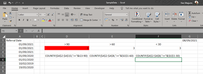
No. of Dates between 30, 60 and 90 days from today ...

[Danni_8oii]

Hi Guys.

I'm trying to calculate the number of dates greater than today's date, I've seemed to have managed the >30 Days, however, I'm struggling with the between 30 & 60, and greater than 90 Days...

No. of Dates from Today >30
No. of Dates from Today <30, but less than 60
No. of Dates from Today >90

I've attached an image of the sample data to assist, but would greatly appreciate any support.

 

[Alex Blakenburg]

Are you sure you don't mean you wanted it aged ?
eg up to 30 days old, 31-60 days old, 61-90 days old, more than 90 days

 

[Toadstool]

Hi Danni_8oli,

Does this do what you want?

Danni_8oli.xlsx
	A	B	C	D	E	F	G
1	Referral Date
2	9/1/2021			>90	>60 <=90	>30 <=60	<=30
3	9/1/2021			0	0	0	7
4	9/1/2021
5	9/1/2021
6	1/1/2020
7	2/10/2019
8	5/19/2020
Sheet1

Cell Formulas
Range	Formula
D3	D3	=COUNTIFS($A$2:$A$9999,">"&TODAY()+90)
E3	E3	=COUNTIFS($A$2:$A$9999,">"&TODAY()+60,$A$2:$A$9999,"<="&G1+90)
F3	F3	=COUNTIFS($A$2:$A$9999,">"&TODAY()+30,$A$2:$A$9999,"<="&H1+60)
G3	G3	=COUNTIFS($A$2:$A$9999,"<="&TODAY()+30)

 

[Alex Blakenburg]

Based on your sample dates, I think having it aged is more likely.
If that is correct try this.
Column B is not used in the formulas and is there as visual validation check only.
I also wante to show that the way I have the formula currently is that I have taken >30 to mean exactly that so it that column would start at 31, > 60 would start at 61 etc.

20210908 Date Aging.xlsx
	A	B	C	D	E	F	G	H	I
1	Referral Date	Aging Days (for verification only)			As at Date --->		8/09/2021
2	1/09/2021	7		>90	>60	>30	0-30	Count Total
3	1/09/2021	7		4	1	2	3	10
4	1/09/2021	7
5	1/08/2021	38
6	1/07/2021	69
7	1/06/2021	99
8	10/07/2021	60
9	1/09/2020	372
10	10/02/2019	941
11	19/05/2019	843
12
13	count --->	10
14
Sheet1

Cell Formulas
Range	Formula
D3	D3	=COUNTIFS($A$2:$A$11,"<"&$G$1-90)
E3	E3	=COUNTIFS($A$2:$A$11,"<"&$G$1-60,$A$2:$A$11,">="&$G$1-90)
F3	F3	=COUNTIFS($A$2:$A$11,"<"&$G$1-30,$A$2:$A$11,">="&$G$1-60)
G3	G3	=COUNTIFS($A$2:$A$11,"<"&$G$1-0,$A$2:$A$11,">="&$G$1-30)
H3	H3	=SUM(D3:G3)
A8	A8	=G1-60
B2:B11	B2	=$G$1-A2
B13	B13	=COUNT(B2:B11)