Nested If Statements (Multiple)

[Excel2021]

Hello,

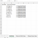
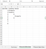
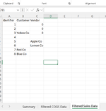
I am having issues getting a complex IF statement working. I have three sheets: "Summary", "Filtered COGS Data" & "Filtered Sales Data". To simplify assume That the "Summary" sheet has 2 columns named "Identifier" and "Customer/Vendor" (Columns A-B) and the other sheets have 3 columns named "Identifier", "Customer" and "Vendor" in columns A-C. The data in these columns are stored from A2:B9 (Headers A1-B1) on the "Summary" and A2:C9 (Headers A1-C1) on the other sheets. I am trying to use IF statements and Xlookups from the "Summary" sheet to both the "Filtered COGS Data" & "Filtered Sales Data" using the "Identifier columns on each sheet (Lookup value will be the identifier column on the summary sheet). The customer or vendor can appear in 1 of the 4 columns across the "Filtered COGS Data" & "Filtered Sales Data" sheets depending on the ERP system data. I am trying to pull whichever column has this into the "Customer/Vendor" column on the summary sheet by eliminating the remaining columns using checks to ensure they <> "" or <>0. My formula which does not work is as follows:

=IF($A2="","",
IF(IF(AND(XLOOKUP($A2,'Filtered COGS Data'!$A$2:$A$9,'Filtered COGS Data'!$B$2:$B$9,0,0,1)<>0,XLOOKUP($A2,'Filtered COGS Data'!$A$2:$A$9,'Filtered COGS Data'!$B$2:$B$9,0,0,1)<>""),XLOOKUP($A2,'Filtered COGS Data'!$A$2:$A$9,'Filtered COGS Data'!$B$2:$B$9,0,0,1),
IF(IF(AND(XLOOKUP($A2,'Filtered Sales Data'!$A$2:$A$9,'Filtered Sales Data'!$B$2:$B$9,0,0,1)<>0,XLOOKUP($A2,'Filtered Sales Data'!$A$2:$A$9,'Filtered Sales Data'!$B$2:$B$9,0,0,1)<>""),XLOOKUP($A2,'Filtered Sales Data'!$A$2:$A$9,'Filtered Sales Data'!$B$2:$B$9,0,0,1),
IF(IF(AND(XLOOKUP($A2,'Filtered Sales Data'!$A$2:$A$9,'Filtered Sales Data'!$C$2:$C$9,0,0,1)<>0,XLOOKUP($A2,'Filtered Sales Data'!$A$2:$A$9,'Filtered Sales Data'!$C$2:$C$9,0,0,1)<>""),XLOOKUP($A2,'Filtered Sales Data'!$A$2:$A$9,'Filtered Sales Data'!$C$2:$C$9,0,0,1),
IF(IF(AND(XLOOKUP($A2,'Filtered COGS Data'!$A$2:$A$9,'Filtered COGS Data'!$C$2:$C$9,0,0,1)<>0,XLOOKUP($A2,'Filtered COGS Data'!$A$2:$A$9,'Filtered COGS Data'!$C$2:$C$9,0,0,1)<>""),XLOOKUP($A2,'Filtered COGS Data'!$A$2:$A$9,'Filtered COGS Data'!$C$2:$C$9,0,0,1),"")))))))))

Thanks

 

[dreid1011]

See if this works for you:

Book1
	A	B
1	Identifier	Customer/Vendor
2	1	Orange Co
3	2	Yellow Co
4	3	Yellow Co
5	4	Orange Co
6	5	Apple Co
7	6	Lemon Co
8	7	Red Co
9	8	Blue Co
Sheet1

Cell Formulas
Range	Formula
B2:B9	B2	=BYROW(A2:A9,LAMBDA(r,LET(x,XLOOKUP(r,$A$2:$A$9,HSTACK('Filtered COGS Data'!$B$2:$C$9,'Filtered Sales Data'!$B$2:$C$9)),y,IF(x=0,"",x),FILTER(y,y<>""))))
Dynamic array formulas.

Book1
	A	B	C
1	Identifier	Customer	Vendor
2	1	Orange Co
3	2	Yellow Co
4	3	0
5	4		Orange Co
6	5	0
7	6
8	7
9	8
Filtered COGS Data

Book1
	A	B	C
1	Identifier	Customer	Vendor
2	1		0
3	2		0
4	3	Yellow Co	0
5	4
6	5		Apple Co
7	6		Lemon Co
8	7	Red Co
9	8	Blue Co
Filtered Sales Data

 

[Excel2021]

See if this works for you:

Book1
	A	B
1	Identifier	Customer/Vendor
2	1	Orange Co
3	2	Yellow Co
4	3	Yellow Co
5	4	Orange Co
6	5	Apple Co
7	6	Lemon Co
8	7	Red Co
9	8	Blue Co
Sheet1

Cell Formulas
Range	Formula
B2:B9	B2	=BYROW(A2:A9,LAMBDA(r,LET(x,XLOOKUP(r,$A$2:$A$9,HSTACK('Filtered COGS Data'!$B$2:$C$9,'Filtered Sales Data'!$B$2:$C$9)),y,IF(x=0,"",x),FILTER(y,y<>""))))
Dynamic array formulas.

Book1
	A	B	C
1	Identifier	Customer	Vendor
2	1	Orange Co
3	2	Yellow Co
4	3	0
5	4		Orange Co
6	5	0
7	6
8	7
9	8
Filtered COGS Data

Book1
	A	B	C
1	Identifier	Customer	Vendor
2	1		0
3	2		0
4	3	Yellow Co	0
5	4
6	5		Apple Co
7	6		Lemon Co
8	7	Red Co
9	8	Blue Co
Filtered Sales Data

Thanks for this. I didn't mention this as I didn't think it would come up but the A "identifier" column on my actual file is already using the filtered formula so I don't think this will work for me. I need a non-array formula for this.

 

[dreid1011]

Why not? Have you tried it? Just replace the "A2:A9" in the BYROW and the XLOOKUP with the formula you have in column A.

 

[Excel2021]

Why not? Have you tried it? Just replace the "A2:A9" in the BYROW and the XLOOKUP with the formula you have in column A.

 

[Excel2021]

I have tried it but the results are not correct when I apply it to my other file. It brings in way more rows than I am expecting. It may be because the columns are not next to each other on the actual file.

 

[dreid1011]

It may be because the columns are not next to each other on the actual file.

Yes, that could do it if your sample is not a true representation of your actual data. And if you didn't adjust the formula provided to fit your data.

 

[Excel2021]

Yes, that could do it if your sample is not a true representation of your actual data. And if you didn't adjust the formula provided to fit your data.

I did adjust it to my file when I tried but it didn't give the results I was expecting.

 

[Excel2021]

I think I figured this out. I changed my existing formula and it seems to be working now.

 

[Excel2021]

I think I figured this out. I changed my existing formula and it seems to be working now.

This is what worked for me.

=IF(A2="","",IF(AND(XLOOKUP(A2,'Filtered COGS Data'!A2:A9,'Filtered COGS Data'!B2:B9,"",0)<>"",XLOOKUP(A2,'Filtered COGS Data'!A2:A9,'Filtered COGS Data'!B2:B9,"",0)<>0),XLOOKUP(A2,'Filtered COGS Data'!A2:A9,'Filtered COGS Data'!B2:B9,"",0),IF(AND(XLOOKUP(A2,'Filtered COGS Data'!A2:A9,'Filtered COGS Data'!C2:C9,"",0)<>"",XLOOKUP(A2,'Filtered COGS Data'!A2:A9,'Filtered COGS Data'!C2:C9,"",0)<>0),XLOOKUP(A2,'Filtered COGS Data'!A2:A9,'Filtered COGS Data'!C2:C9,"",0),IF(AND(XLOOKUP(A2,'Filtered Sales Data'!A2:A9,'Filtered Sales Data'!B2:B9,"",0)<>"",XLOOKUP(A2,'Filtered Sales Data'!A2:A9,'Filtered Sales Data'!B2:B9,"",0)<>0),XLOOKUP(A2,'Filtered Sales Data'!A2:A9,'Filtered Sales Data'!B2:B9,"",0),IF(AND(XLOOKUP(A2,'Filtered Sales Data'!A2:A9,'Filtered Sales Data'!C2:C9,"",0)<>"",XLOOKUP(A2,'Filtered Sales Data'!A2:A9,'Filtered Sales Data'!C2:C9,"",0)<>0),XLOOKUP(A2,'Filtered Sales Data'!A2:A9,'Filtered Sales Data'!C2:C9,"",0),)))))