Named Range not working

[markh9999]

Hello. I am having a lot of trouble doing a very simple thing. I have stripped the problem down to it's bare bones.

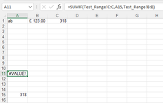
Basically, I have a named range called Test_Range which is just cells A1 to A3. A1 is just text, A2 contains a Currency value (in £) of £123 and A3 contains a value of 318.

In Cell A15 I have the number 318 and in cell A11 I have this formula:

=SUMIF(Test_Range!C:C,A15,Test_Range!B:B).

I would expect this to return 123 but instead it brings up a file directory showing the directory that the workbook is saved in?

If I use the 'Evaluate function' option it's not even recognising the cell A15 as having 318 in it?

If I use actual ranges rather than a named range it works fine.

Any ideas?

 

[Joe4]

Basically, I have a named range called Test_Range which is just cells A1 to A3

That does not seem right, when the data you want to sum is in columns B and C.
What exactly is "Test_Range" set to? A1:A3 does not seem like it would work.

 

[RoryA]

You can't refer to cells in a named range the same way you use a sheet name. I don't really understand why you would do what you're describing so it's hard to suggest your best alternative, but I imagine you will need INDEX.

 

[felixstraube]

This syntax is for the sheet name, not for a named range:

"Test_Range!C:C"

This means sheet "Test_Range" column C (complete column C)

 

[markh9999]

Thanks everyone, I think I have confused you all (and myself).

Forget everything above.

What I am trying to do is this:

I have a named range called TEST which has columns A to G (TEST in on Sheet2).

I want a formula on Sheet1 that looks at the number in Cell B11 and if that number occurs at all in Column G of TEST then add the corresponding value in Column D of TEST. There may be
lots of entries that match or none at all (formula should then return zero).

Hope that makes more sense?

 

[Joe4]

Which version of Excel are you using? I suggest that you update your Account details (or click your user name at the top right of the forum) so helpers always know what Excel version(s) & platform(s) you are using as the best solution often varies by version. (Don’t forget to scroll down & ‘Save’).

I don't think the named range serves any purpose here, since you are just looking up into a single column and returning the value from another column.

A formula like this should do what you want, provided you are on a version of Excel that has the XLOOKUP function:

=XLOOKUP(B11,Sheet2!G:G,Sheet2!D:D,0)

However, what exactly do you want to happen if there are multiple matches?
Do you want ALL of them returned?
If so, and you have the FILTER function, you could use:

=FILTER(Sheet2!D:D,Sheet2!G:G=B11,0)

 

[markh9999]

Which version of Excel are you using? I suggest that you update your Account details (or click your user name at the top right of the forum) so helpers always know what Excel version(s) & platform(s) you are using as the best solution often varies by version. (Don’t forget to scroll down & ‘Save’).

I don't think the named range serves any purpose here, since you are just looking up into a single column and returning the value from another column.

A formula like this should do what you want, provided you are on a version of Excel that has the XLOOKUP function:

=XLOOKUP(B11,Sheet2!G:G,Sheet2!D:D,0)

However, what exactly do you want to happen if there are multiple matches?
Do you want ALL of them returned?
If so, and you have the FILTER function, you could use:

=FILTER(Sheet2!D:D,Sheet2!G:G=B11,0)

 

[markh9999]

Thank you Joe - I didn't know about the filter command!

 

[Joe4]

You are welcome.

Note. When you mark a post as the solution, please mark the actual post that contains the solution, and not your own post quoting the post with the solution.
I have updated this for you on this thread.