Name Manager Help

[AaronFi]

Hello, first time poster here!

I am looking to use the name manager to define names where the results will update whenever I refresh the table it's referencing.

Here's the table:
Column A are categories
Column B are part numbers
Column C are descriptions
Column D are prices

Is it possible to create a new name where the name is one of the product categories (looks at column A and pulls in the correct rows) and the list it generates is a list of descriptions (column C)?

 

[JGordon11]

An example for
Table named Table1 (needs to be a formal excel table, CTRL-T to turn your data into a table if is not one)
Category column labelled Category
Description column labelled Desc
Category of interest Valve

Go to name manager
Name: Valve
Formula:

=FILTER(Table1[Desc], Table1[Category]="Valve")

Then if you type =Valve in a cell it will spill all the valve descriptions from Table1

Change Table1, Category, Desc, and Valve as needed to match your setup

 

[AaronFi]

An example for
Table named Table1 (needs to be a formal excel table, CTRL-T to turn your data into a table if is not one)
Category column labelled Category
Description column labelled Desc
Category of interest Valve

Go to name manager
Name: Valve
Formula:

=FILTER(Table1[Desc], Table1[Category]="Valve")

Then if you type =Valve in a cell it will spill all the valve descriptions from Table1

Change Table1, Category, Desc, and Valve as needed to match your setup

Thanks for responding! I believe I am almost there, but for some reason the formula is not creating a list of options. Here's the formula I ended up creating:

=FILTER(Catalog[Description], Catalog[IPS_Categories]="Motherboard")

Category column labelled IPS_Categories
Description column labelled Description
Category of interest Motherboard

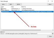
The formula didn't error out but the value is doing nothing more than posting as {...}. Any ideas on what I am doing wrong?

 

[AaronFi]

Thanks for responding! I believe I am almost there, but for some reason the formula is not creating a list of options. Here's the formula I ended up creating:

=FILTER(Catalog[Description], Catalog[IPS_Categories]="Motherboard")

Category column labelled IPS_Categories
Description column labelled Description
Category of interest Motherboard

The formula didn't error out but the value is doing nothing more than posting as {...}. Any ideas on what I am doing wrong?

One more interesting note - if I use the same exact formula in a cell to generate a list, the formula works and displays everything correctly.
So, inside of name manager, all I get is {...}
Typed into a cell, I get a list of 5 items, which is as expected.

 

[JGordon11]

I'm not sure why it is not working for you. It works here

Book2
	A	B	C	D	E	F	G
1	IPS_Categories	Part No	Description	Price
2	Gasket	7370	S	520.13		B
3	Spring	6471	K	161.36		P
4	Motherboard	3832	B	413.01		D
5	Hose	4594	M	122.88		H
6	Valve	1925	G	186.82		Q
7	Motherboard	1779	P	920.06		I
8	Hose	2074	O	846.86
9	Valve	3887	C	449.98
10	Motherboard	8456	D	804.34
11	Belt	8757	R	926.61
12	Belt	2890	F	115.93
13	Valve	9011	T	445.55
14	Motherboard	4842	H	782.85
15	Belt	9360	A	494.21
16	Motherboard	9947	Q	955.21
17	Motherboard	1923	I	646.13
18	Valve	8939	L	511.42
19	Spring	2420	J	279.06
20	Hose	2116	N	403.25
21	Valve	3333	E	255.03
22
Sheet2

Cell Formulas
Range	Formula
F2:F7	F2	=Motherboard
Dynamic array formulas.

 

[Fluff]

So, inside of name manager, all I get is {...}

That is what you will get, as the name manager doesn't know what the values are until the formula calculates.

 

[AaronFi]

I'm not sure why it is not working for you. It works here

View attachment 76295

Book2
	A	B	C	D	E	F	G
1	IPS_Categories	Part No	Description	Price
2	Gasket	7370	S	520.13		B
3	Spring	6471	K	161.36		P
4	Motherboard	3832	B	413.01		D
5	Hose	4594	M	122.88		H
6	Valve	1925	G	186.82		Q
7	Motherboard	1779	P	920.06		I
8	Hose	2074	O	846.86
9	Valve	3887	C	449.98
10	Motherboard	8456	D	804.34
11	Belt	8757	R	926.61
12	Belt	2890	F	115.93
13	Valve	9011	T	445.55
14	Motherboard	4842	H	782.85
15	Belt	9360	A	494.21
16	Motherboard	9947	Q	955.21
17	Motherboard	1923	I	646.13
18	Valve	8939	L	511.42
19	Spring	2420	J	279.06
20	Hose	2116	N	403.25
21	Valve	3333	E	255.03
22
Sheet2

Cell Formulas
Range	Formula
F2:F7	F2	=Motherboard
Dynamic array formulas.

If I spill the results into a spreadsheet like you did, it works for me too.

It's when I use the name manager to generate results that nothing gets picked up.

 

[AaronFi]

That is what you will get, as the name manager doesn't know what the values are until the formula calculates.

Then maybe my problem is further downstream. The reason I am doing this is I need to use data validation to create a drop-down list of products by category. I am trying to use the indirect function to reference the defined names to create the drop-down list. Can I not use the names in this manner?

 

[Fluff]

Can I not use the names in this manner?

No you can't, but if you put the formula in F2 (for instance) then you can refer to that cell in the data validation using =F2#

 

[AaronFi]

No you can't, but if you put the formula in F2 (for instance) then you can refer to that cell in the data validation using =F2#

This worked! I created a new sheet within the workbook, named each column by what would be housed in that column, used each column to spill the results of each category, and bingo, I'm up and running.

Thank you to both @JGordon11 and @Fluff for the assistance!