Multiple IF with SumProduct

volsfan210

New Member
Joined
Jul 24, 2024
Messages
13
Office Version
  1. 365
Hi -

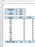
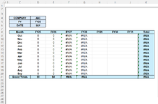
Currently have summary data that is summed by FY and Month and below is the formula. (TEST 6 Image is the Summary)

=SUMPRODUCT(('INITAL ENTRY DATA RAW'!$L$1:$BD$1='PHASE SUMMARY'!D$6)*('INITAL ENTRY DATA RAW'!$L$2:$BD$2='PHASE SUMMARY'!$C7)*'INITAL ENTRY DATA RAW'!$L$4:$BD$1999)

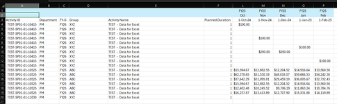
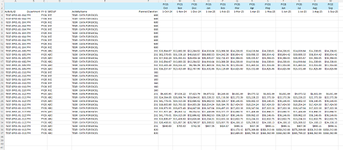
( TEST 5 Image is the details))In Column D of the inital entry file there are two codes "ABC" and "XYZ" that represent each line of the data. I would like the summary to be able to give me the totals on just the ABC, XYZ and overall.

Is there a way I can accomplish this
 

Attachments

  • Test 5.png
    Test 5.png
    63.8 KB · Views: 18
  • Test 6.png
    Test 6.png
    14.3 KB · Views: 18

Excel Facts

Ambidextrous Undo
Undo last command with Ctrl+Z or Alt+Backspace. If you use the Undo icon in the QAT, open the drop-down arrow to undo up to 100 steps.
Perhaps something along these lines:

Excel Formula:
=SUMPRODUCT(('INITAL ENTRY DATA RAW'!$L$1:$BD$1='PHASE SUMMARY'!D$6)*('INITAL ENTRY DATA RAW'!$L$2:$BD$2='PHASE SUMMARY'!$C7)*IF(ISBLANK('PHASE SUMMARY'!$D$4),1,('INITAL ENTRY DATA RAW'!$D$4:$D$1999='PHASE SUMMARY'!$D$4))*'INITAL ENTRY DATA RAW'!$L$4:$BD$1999)

This will return the group total for the specified code in cell D4; or, if D4 is blank, it will return the overall total.

Also, with MS365, you could try using a single cell array formula to spill the results for the entire summary. For example:

Excel Formula:
=LET(
    hdr, 'INITAL ENTRY DATA RAW'!L1:BD1 & 'INITAL ENTRY DATA RAW'!L2:BD2,
    grp, 'INITAL ENTRY DATA RAW'!D4:D1999,
    val, 'INITAL ENTRY DATA RAW'!L4:BD1999,
    code, 'PHASE SUMMARY'!D4,
    MAP('PHASE SUMMARY'!D6:E6 & 'PHASE SUMMARY'!C7:C18, LAMBDA(ym, LET(
        rng, XLOOKUP(ym, hdr, val, ""),
        IF(ROWS(rng)=1, 0, IF(ISBLANK(code), SUM(rng), SUMIFS(rng, grp, code)))))
    )
)
 
Upvote 0
Perhaps something along these lines:

Excel Formula:
=SUMPRODUCT(('INITAL ENTRY DATA RAW'!$L$1:$BD$1='PHASE SUMMARY'!D$6)*('INITAL ENTRY DATA RAW'!$L$2:$BD$2='PHASE SUMMARY'!$C7)*IF(ISBLANK('PHASE SUMMARY'!$D$4),1,('INITAL ENTRY DATA RAW'!$D$4:$D$1999='PHASE SUMMARY'!$D$4))*'INITAL ENTRY DATA RAW'!$L$4:$BD$1999)

This will return the group total for the specified code in cell D4; or, if D4 is blank, it will return the overall total.

Also, with MS365, you could try using a single cell array formula to spill the results for the entire summary. For example:

Excel Formula:
=LET(
    hdr, 'INITAL ENTRY DATA RAW'!L1:BD1 & 'INITAL ENTRY DATA RAW'!L2:BD2,
    grp, 'INITAL ENTRY DATA RAW'!D4:D1999,
    val, 'INITAL ENTRY DATA RAW'!L4:BD1999,
    code, 'PHASE SUMMARY'!D4,
    MAP('PHASE SUMMARY'!D6:E6 & 'PHASE SUMMARY'!C7:C18, LAMBDA(ym, LET(
        rng, XLOOKUP(ym, hdr, val, ""),
        IF(ROWS(rng)=1, 0, IF(ISBLANK(code), SUM(rng), SUMIFS(rng, grp, code)))))
    )
)
Perfect! Using the ISBlank gives us exactly what we needed!
 
Upvote 0
One other thing that would be a nice to have but not sure if possible would be the following

can you take the formula below and add in another couple toggles.

So say in D21 and D22 I have the month and FY reflected and I only want it to populate the summary to that Month and FY in D21 & D22.

i.e D21 (DEC) and D22 (FY25). So the summary chart would only give me Oct,Nov,Dec. But if I wanted to change the month to FEB it would then show Oct,Nov,Dec,Jan,Feb

=SUMPRODUCT(('INITAL ENTRY DATA RAW'!$L$1:$BD$1='PHASE SUMMARY'!D$6)*('INITAL ENTRY DATA RAW'!$L$2:$BD$2='PHASE SUMMARY'!$C7)*IF(ISBLANK('PHASE SUMMARY'!$D$4),1,('INITAL ENTRY DATA RAW'!$D$4:$D$1999='PHASE SUMMARY'!$D$4))*'INITAL ENTRY DATA RAW'!$L$4:$BD$1999)
 
Upvote 0
If D21 equals "Dec" and D22 equals "FY25", would the FY26 column (E7:E18) return no data (zeros) for the entire year? Likewise, if D21 equals "Dec" and D22 equals "FY26", would the FY25 column (D7:D18) return data for the entire year (every month), and the FY26 column would only return data up to Dec (Oct, Nov, Dec)?

If so, try the following in cell D7 and copy down/across:

Excel Formula:
=IF(OR(MATCH(D$6,$D$6:$E$6,0)<MATCH($D$22,$D$6:$E$6,0),AND(MATCH(D$6,$D$6:$E$6,0)=MATCH($D$22,$D$6:$E$6,0),MATCH($C7,$C$7:$C$18,0)<=MATCH($D$21,$C$7:$C$18,0))),SUMPRODUCT(('INITAL ENTRY DATA RAW'!$L$1:$BD$1=D$6)*('INITAL ENTRY DATA RAW'!$L$2:$BD$2=$C7)*IF(ISBLANK($D$4),1,('INITAL ENTRY DATA RAW'!$D$4:$D$1999=$D$4))*'INITAL ENTRY DATA RAW'!$L$4:$BD$1999),0)

Please note, this formula is backwards-compatible for older versions of Excel. There are newer functions/methods available for MS365 that could also be used.

If I misinterpreted what you were asking, please provide an updated sample dataset with expected results. Cheers!

Hi -

Attached is updated images for you..

What I would like to have happen is when I have the toggles populated if gives me the monthly numbers up until the FY/Data identified. If I don't have a date or FY identified then I want the table to fully populated as you can see in the image I have data past Sep FY25.
 

Attachments

  • Test 7.png
    Test 7.png
    30.6 KB · Views: 3
  • Test 8.png
    Test 8.png
    233.2 KB · Views: 3
Upvote 0
Try the following in cell D9 and copy down/across:

Excel Formula:
=IF(AND(ISBLANK($D$5),MATCH($C9,$C$9:$C$20,0)>IF(ISBLANK($D$6),ROWS($C$9:$C$20),MATCH($D$6,$C$9:$C$20,0))),0,IF(OR(MATCH(D$8,$D$8:$E$8,0)<IF(ISBLANK($D$5),COLUMNS($D$8:$E$8),MATCH($D$5,$D$8:$E$8,0)),AND(MATCH(D$8,$D$8:$E$8,0)=IF(ISBLANK($D$5),COLUMNS($D$8:$E$8),MATCH($D$5,$D$8:$E$8,0)),MATCH($C9,$C$9:$C$20,0)<=IF(ISBLANK($D$6),ROWS($C$9:$C$20),MATCH($D$6,$C$9:$C$20,0)))),SUMPRODUCT(('INITAL ENTRY DATA RAW'!$L$1:$BD$1=D$8)*('INITAL ENTRY DATA RAW'!$L$2:$BD$2=$C9)*IF(ISBLANK($D$4),1,('INITAL ENTRY DATA RAW'!$D$4:$D$1999=$D$4))*'INITAL ENTRY DATA RAW'!$L$4:$BD$1999),0))

Or, simplified with LET:

Excel Formula:
=LET(
    years, $D$8:$E$8,
    y, IF(ISBLANK($D$5),COLUMNS(years),XMATCH($D$5,years)),
    c, XMATCH(D$8,years),
    months, $C$9:$C$20,
    m, IF(ISBLANK($D$6),ROWS(months),XMATCH($D$6,months)),
    r, XMATCH($C9,months),
    IF(AND(ISBLANK($D$5),r>m),0,IF(OR(c<y,AND(c=y,r<=m)),SUMPRODUCT(('INITAL ENTRY DATA RAW'!$L$1:$BD$1=D$8)*('INITAL ENTRY DATA RAW'!$L$2:$BD$2=$C9)*IF(ISBLANK($D$4),1,('INITAL ENTRY DATA RAW'!$D$4:$D$1999=$D$4))*'INITAL ENTRY DATA RAW'!$L$4:$BD$1999),0))
)

Or, as a spilled array with MAP:

Excel Formula:
=LET(
    years, D8:E8,
    y, IF(ISBLANK(D5), COLUMNS(years), XMATCH(D5, years)),
    months, C9:C20,
    m, IF(ISBLANK(D6), ROWS(months), XMATCH(D6, months)),
    hdr, 'INITAL ENTRY DATA RAW'!L1:BD1 & 'INITAL ENTRY DATA RAW'!L2:BD2,
    grp, 'INITAL ENTRY DATA RAW'!D4:D1999,
    val, 'INITAL ENTRY DATA RAW'!L4:BD1999,
    MAP(years & months, IF({1}, SEQUENCE(ROWS(months)), years), IF({1}, SEQUENCE(, COLUMNS(years)), months), LAMBDA(ym,r,c,
        IF(AND(ISBLANK(D5), r>m), 0, IF(OR(c<y, AND(c=y, r<=m)),
            LET(rng, XLOOKUP(ym, hdr, val, ""), IF(ROWS(rng)=1, 0, IF(ISBLANK(D4), SUM(rng), SUMIFS(rng, grp, D4)))), 0)))
    )
)

I may have over-complicated it, but it seems to work anyway.
Thank you!!!

Hate to ask but if I wanted to extend the FY to FY31 based off attached image is that doable?
 

Attachments

  • Test 9.png
    Test 9.png
    59.1 KB · Views: 2
Upvote 0
Just update all references to the fiscal year range from $D$8:$E$8 to $D$8:$J$8...

Excel Formula:
=IF(AND(ISBLANK($D$5),MATCH($C9,$C$9:$C$20,0)>IF(ISBLANK($D$6),ROWS($C$9:$C$20),MATCH($D$6,$C$9:$C$20,0))),0,IF(OR(MATCH(D$8,$D$8:$J$8,0)<IF(ISBLANK($D$5),COLUMNS($D$8:$J$8),MATCH($D$5,$D$8:$J$8,0)),AND(MATCH(D$8,$D$8:$J$8,0)=IF(ISBLANK($D$5),COLUMNS($D$8:$J$8),MATCH($D$5,$D$8:$J$8,0)),MATCH($C9,$C$9:$C$20,0)<=IF(ISBLANK($D$6),ROWS($C$9:$C$20),MATCH($D$6,$C$9:$C$20,0)))),SUMPRODUCT(('INITAL ENTRY DATA RAW'!$L$1:$BD$1=D$8)*('INITAL ENTRY DATA RAW'!$L$2:$BD$2=$C9)*IF(ISBLANK($D$4),1,('INITAL ENTRY DATA RAW'!$D$4:$D$1999=$D$4))*'INITAL ENTRY DATA RAW'!$L$4:$BD$1999),0))

For the other two examples where I used LET, you would only need to update the years variable.
 
Upvote 0

Forum statistics

Threads
1,222,905
Messages
6,168,949
Members
452,227
Latest member
sam1121

We've detected that you are using an adblocker.

We have a great community of people providing Excel help here, but the hosting costs are enormous. You can help keep this site running by allowing ads on MrExcel.com.
Allow Ads at MrExcel

Which adblocker are you using?

Disable AdBlock

Follow these easy steps to disable AdBlock

1)Click on the icon in the browser’s toolbar.
2)Click on the icon in the browser’s toolbar.
2)Click on the "Pause on this site" option.
Go back

Disable AdBlock Plus

Follow these easy steps to disable AdBlock Plus

1)Click on the icon in the browser’s toolbar.
2)Click on the toggle to disable it for "mrexcel.com".
Go back

Disable uBlock Origin

Follow these easy steps to disable uBlock Origin

1)Click on the icon in the browser’s toolbar.
2)Click on the "Power" button.
3)Click on the "Refresh" button.
Go back

Disable uBlock

Follow these easy steps to disable uBlock

1)Click on the icon in the browser’s toolbar.
2)Click on the "Power" button.
3)Click on the "Refresh" button.
Go back
Back
Top