Multiple Conditional Dropdown list, without Duplicate

[Shayanan]

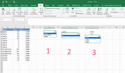
I have a Table, with 3 column. In picture I showed what I want. I need 3 dropdown list that depend each.
List 1= list cul-1 (without duplicate).
list 2= everything in Cul-2 related to return of list 1 (without duplicate).
list 3= everything in Cul-3 related to return of list 2 (without duplicate).

In the picture, column "J" is what I want.

 

[Peter_SSs]

Try something like this.
Helper columns L:N could be hidden if you want.

Shayanan.xlsm
	A	B	C	D	E	F	G	H	I	J	K	L	M	N
1												$L$3:$L$5	$M$3:$M$4	$N$3:$N$6
2	Game	96	17000			Game		2
3	Game	96	17500									Game	96	17000
4	Game	96	18000									Productivity	2	17500
5	Game	96	18500									Utility		18000
6	Game	2	17000											18500
7	Game	2	17500
8	Game	2	18000
9	Game	2	18500
10	Productivity	124	10000
11	Productivity	124	10500
12	Productivity	124	11000
13	Utility	18	21000
14	Utility	18	22000
15	Utility	18	23000
16
Sheet1

Cell Formulas
Range	Formula
L1	L1	=ADDRESS(3,COLUMN())&":"&ADDRESS(2+COUNTIF(L3:L21,"?*"),COLUMN())
M1:N1	M1	=ADDRESS(3,COLUMN())&":"&ADDRESS(2+MAX(COUNT(M3:M21),1),COLUMN())
L3:L16	L3	=IFERROR(INDEX(A$2:A$20,MATCH(0,INDEX(COUNTIF(L$2:L2,A$2:A$20)+(A$2:A$20=""),0),0)),"")
M3:M16	M3	=IF($F$2="","",IFERROR(INDEX(B$2:B$20,AGGREGATE(15,6,(ROW(B$2:B$20)-ROW(B$2)+1)/((A$2:A$20=F$2)*(ISNA(MATCH(B$2:B$20,M$2:M2,0)))),1)),""))
N3:N16	N3	=IF(H$2="","",IFERROR(INDEX(C$2:C$20,AGGREGATE(15,6,(ROW(C$2:C$20)-ROW(C$2)+1)/((B$2:B$20=H$2)*(ISNA(MATCH(C$2:C$20,N$2:N2,0)))),1)),""))

Cells with Data Validation
Cell	Allow	Criteria
F2	List	=INDIRECT($L$1)
H2	List	=INDIRECT($M$1)
J2	List	=INDIRECT($N$1)

 

[Shayanan]

Try something like this.
Helper columns L:N could be hidden if you want.

Shayanan.xlsm
	A	B	C	D	E	F	G	H	I	J	K	L	M	N
1												$L$3:$L$5	$M$3:$M$4	$N$3:$N$6
2	Game	96	17000			Game		2
3	Game	96	17500									Game	96	17000
4	Game	96	18000									Productivity	2	17500
5	Game	96	18500									Utility		18000
6	Game	2	17000											18500
7	Game	2	17500
8	Game	2	18000
9	Game	2	18500
10	Productivity	124	10000
11	Productivity	124	10500
12	Productivity	124	11000
13	Utility	18	21000
14	Utility	18	22000
15	Utility	18	23000
16
Sheet1

Cell Formulas
Range	Formula
L1	L1	=ADDRESS(3,COLUMN())&":"&ADDRESS(2+COUNTIF(L3:L21,"?*"),COLUMN())
M1:N1	M1	=ADDRESS(3,COLUMN())&":"&ADDRESS(2+MAX(COUNT(M3:M21),1),COLUMN())
L3:L16	L3	=IFERROR(INDEX(A$2:A$20,MATCH(0,INDEX(COUNTIF(L$2:L2,A$2:A$20)+(A$2:A$20=""),0),0)),"")
M3:M16	M3	=IF($F$2="","",IFERROR(INDEX(B$2:B$20,AGGREGATE(15,6,(ROW(B$2:B$20)-ROW(B$2)+1)/((A$2:A$20=F$2)*(ISNA(MATCH(B$2:B$20,M$2:M2,0)))),1)),""))
N3:N16	N3	=IF(H$2="","",IFERROR(INDEX(C$2:C$20,AGGREGATE(15,6,(ROW(C$2:C$20)-ROW(C$2)+1)/((B$2:B$20=H$2)*(ISNA(MATCH(C$2:C$20,N$2:N2,0)))),1)),""))

Cells with Data Validation
Cell	Allow	Criteria
F2	List	=INDIRECT($L$1)
H2	List	=INDIRECT($M$1)
J2	List	=INDIRECT($N$1)

View attachment 31981

thanks for your help. its work but there is a little problem.

in column-B , if utility=18 become utility=96, so we have 96 common in game and utility and it became sub of irrelevant parent.

 

[Peter_SSs]

but there is a little problem.

in column-B , if utility=18 become utility=96, so we have 96 common in game and utility and it became sub of irrelevant parent.

I'm not sure that I directly understand what you have written, but I think I can see the problem anyway. See if this is better

Shayanan.xlsm
	A	B	C	D	E	F	G	H	I	J	K	L	M	N
1												$L$3:$L$5	$M$3:$M$3	$N$3:$N$5
2	Game	96	17000			Utility		96
3	Game	96	17500									Game	96	21000
4	Game	96	18000									Productivity		22000
5	Game	96	18500									Utility		23000
6	Game	2	17000
7	Game	2	17500
8	Game	2	18000
9	Game	2	18500
10	Productivity	124	10000
11	Productivity	124	10500
12	Productivity	124	11000
13	Utility	96	21000
14	Utility	96	22000
15	Utility	96	23000
16
Sheet1

Cell Formulas
Range	Formula
L1	L1	=ADDRESS(3,COLUMN())&":"&ADDRESS(2+COUNTIF(L3:L21,"?*"),COLUMN())
M1:N1	M1	=ADDRESS(3,COLUMN())&":"&ADDRESS(2+MAX(COUNT(M3:M21),1),COLUMN())
L3:L16	L3	=IFERROR(INDEX(A$2:A$20,MATCH(0,INDEX(COUNTIF(L$2:L2,A$2:A$20)+(A$2:A$20=""),0),0)),"")
M3:M16	M3	=IF($F$2="","",IFERROR(INDEX(B$2:B$20,AGGREGATE(15,6,(ROW(B$2:B$20)-ROW(B$2)+1)/((A$2:A$20=F$2)*(ISNA(MATCH(B$2:B$20,M$2:M2,0)))),1)),""))
N3:N16	N3	=IF(H$2="","",IFERROR(INDEX(C$2:C$20,AGGREGATE(15,6,(ROW(C$2:C$20)-ROW(C$2)+1)/((B$2:B$20=H$2)*(A$2:A$20=F$2)*(ISNA(MATCH(C$2:C$20,N$2:N2,0)))),1)),""))

Cells with Data Validation
Cell	Allow	Criteria
F2	List	=INDIRECT($L$1)
H2	List	=INDIRECT($M$1)
J2	List	=INDIRECT($N$1)

 

[Shayanan]

I'm not sure that I directly understand what you have written, but I think I can see the problem anyway. See if this is better

Shayanan.xlsm
	A	B	C	D	E	F	G	H	I	J	K	L	M	N
1												$L$3:$L$5	$M$3:$M$3	$N$3:$N$5
2	Game	96	17000			Utility		96
3	Game	96	17500									Game	96	21000
4	Game	96	18000									Productivity		22000
5	Game	96	18500									Utility		23000
6	Game	2	17000
7	Game	2	17500
8	Game	2	18000
9	Game	2	18500
10	Productivity	124	10000
11	Productivity	124	10500
12	Productivity	124	11000
13	Utility	96	21000
14	Utility	96	22000
15	Utility	96	23000
16
Sheet1

Cell Formulas
Range	Formula
L1	L1	=ADDRESS(3,COLUMN())&":"&ADDRESS(2+COUNTIF(L3:L21,"?*"),COLUMN())
M1:N1	M1	=ADDRESS(3,COLUMN())&":"&ADDRESS(2+MAX(COUNT(M3:M21),1),COLUMN())
L3:L16	L3	=IFERROR(INDEX(A$2:A$20,MATCH(0,INDEX(COUNTIF(L$2:L2,A$2:A$20)+(A$2:A$20=""),0),0)),"")
M3:M16	M3	=IF($F$2="","",IFERROR(INDEX(B$2:B$20,AGGREGATE(15,6,(ROW(B$2:B$20)-ROW(B$2)+1)/((A$2:A$20=F$2)*(ISNA(MATCH(B$2:B$20,M$2:M2,0)))),1)),""))
N3:N16	N3	=IF(H$2="","",IFERROR(INDEX(C$2:C$20,AGGREGATE(15,6,(ROW(C$2:C$20)-ROW(C$2)+1)/((B$2:B$20=H$2)*(A$2:A$20=F$2)*(ISNA(MATCH(C$2:C$20,N$2:N2,0)))),1)),""))

Cells with Data Validation
Cell	Allow	Criteria
F2	List	=INDIRECT($L$1)
H2	List	=INDIRECT($M$1)
J2	List	=INDIRECT($N$1)

View attachment 32026

Thanks a lot. You correct what problem I've got.

 

[Peter_SSs]

You're welcome. Thanks for the confirmation.

 

[Coops01]

Hi - following this thread worked very nicely for a similar problem I had - thank you. However, if I wanted the dropdown data validation on a different tab, how do I use the INDIRECT() function to return the contents of a desired array kept on a separate tab please?

The desirable product I need is for a table to be maintained on one tab, with the input/dropdown selection forms on another tab.