Monthly Vs Quarterly

[arnabmit]

Hi,

I have 3 tables, one with sales figures, another a HeadCount table, another a calendar table.

Calendar:
Date Month Quarter
4/1/19 Apr Q1
4/2/19 Apr Q1
4/3/19 Apr Q1
...


SalesPerson HeadCount
Month HC
Apr 12
May 10
Jun 9
Jul 10
...


Sales:
EmpID Date Qty_Sold
1234 4/1/19 3
2345 4/1/19 2
3456 4/1/19 4
...

I want to find out total SumOfQty_Sales/SalesPersons to get AvgQtySoldPerPerson month wise.

The place where I am getting stuck is that when I select the Q1 in the slicer, instead of month.

I want it to give me total Qty_Sold for the quarter / HC for Jun (quarter closing HC). Instead it is giving me total Qty_Sold / total HC.

 

[CA_Punit]

This is a simple example of your result sought. I want your report layout picture so that i can understand where is the probelm in Slicer???

aug20 maa bhagwati.xlsx
	A	B	C	D	E	F	G	H	I	J	K	L
1	Month	HC					Sales
2	April	12					EmployeeID	Date	Quantity Sold
3	May	10					1234	01-04-2019	3
4	June	9					2345	02-04-2019	2
5	July	10					3456	03-04-2019	3
6							1111	01-05-2019	1
7							2222	02-05-2019	32
8							3333	03-05-2019	1
9
10
11
12
13	MonthWise Average Quantity Sold
14
15	April	0.67
16	May	3.40
17	June	-
18	July	-
19
20
Sheet2

Cell Formulas
Range	Formula
B15:B18	B15	=SUM(IF(TEXT($H$3:$H$8,"mmmM")=A15,$I$3:$I$8))/SUM(IF($A$15:$A$18=A2,$B$2:$B$5))

 

[arnabmit]

This is a simple example of your result sought. I want your report layout picture so that i can understand where is the probelm in Slicer???

Hi,

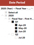
These are the tables and result sample I am working with. The date slicer I will be using is attached as an image

Date Test.xlsx
	A	B	C	D	E	F	G	H	I	J	K
1	Date	Month	Qtr		Month	HC		EmpID	Date	Qty_Sold
2	1-Apr-19	Apr	Q1		Apr	12		1234	1-Apr-19	5
3	2-Apr-19	Apr	Q1		May	10		2345	5-Apr-19	6
4	3-Apr-19	Apr	Q1		Jun	9		3456	5-May-19	7
5	4-Apr-19	Apr	Q1		Jul	10		4567	6-Jun-19	4
6	5-Apr-19	Apr	Q1		Aug	11		5678	7-Jul-19	3
7	…				Sep	12		6789	8-Aug-19	9
8	1-May-19	May	Q1		Oct	10		7890	9-Sep-19	5
9	1-Jun-19	Jun	Q1		Nov	9		8901	10-Oct-19	4
10	1-Jul-19	Jul	Q2		Dec	10		9012	11-Nov-19	8
11	1-Aug-19	Aug	Q2					1234	4-Apr-19	6
12	1-Sep-19	Sep	Q2					2345	4-May-19	2
13	1-Oct-19	Oct	Q3					3456	4-Jun-19	4
14	1-Nov-19	Nov	Q3					4567	4-Jul-19	6
15	1-Dec-19	Dec	Q3					5678	4-Aug-19	5
16								6789	4-Sep-19	7
17	Result							7890	4-Oct-19	9
18								8901	4-Nov-19	3
19		Period	HC	Qty	Qty/HC			9012	4-Dec-19	1
20		Apr	12	22	1.8			1234	25-Apr-19	5
21		May	10	11	1.1			2345	25-May-19	2
22		Jun	9	12	1.3			3456	25-Jun-19	4
23		Q1	9	45	5.0			4567	25-Jul-19	6
24		Jul	10	15	1.5			5678	25-Aug-19	9
25		Aug	11	23	2.1			6789	25-Sep-19	7
26		Sep	12	19	1.6			7890	25-Oct-19	8
27		Q2	12	57	4.8			8901	25-Nov-19	5
28								9012	25-Dec-19	8
29
Sheet1

Cell Formulas
Range	Formula
B8:B15,B2:B6	B2	=TEXT(A2,"mmm")
C8:C15,C2:C6	C2	=CHOOSE(ROUNDUP(MONTH(A2)/3,0),"Q4","Q1","Q2","Q3")
C23,C27	C23	=C22
D23,D27	D23	=SUM(D20:D22)
E20:E27	E20	=D20/C20

 

[CA_Punit]

I don't think it can be done through Slicer. Instead if you want it can be done through Formula.

 

[arnabmit]

I don't think it can be done through Slicer. Instead if you want it can be done through Formula.

It would be great if you can help me implement it using M code.

 

[Bo_Ry]

Create Table HC and Qty
Then

let
    Source = Excel.CurrentWorkbook(){[Name="Qty"]}[Content],
    #"Changed Type" = Table.TransformColumnTypes(Source,{{"Date", type date}}),
    AddedMonthName = Table.AddColumn(#"Changed Type", "Period", each Date.ToText([Date],"MMM")),
    AddedQuarter = Table.AddColumn(AddedMonthName, "Quarter", each Number.ToText(Number.Mod(3+Number.IntegerDivide(Date.Month([Date])-1,3),4)+1,"\Q0")),
    #"Grouped Rows" = Table.Group(AddedQuarter, {"Quarter", "Period"}, {{"Qty", each List.Sum([Qty_Sold]), type number}}),
    #"Merged Queries" = Table.NestedJoin(#"Grouped Rows", {"Period"}, Excel.CurrentWorkbook(){[Name="HC"]}[Content], {"Month"}, "Grouped", JoinKind.LeftOuter),
    #"Expanded Grouped" = Table.ExpandTableColumn(#"Merged Queries", "Grouped", {"HC"}, {"HC"}),
    #"Grouped Rows1" = Table.Group(#"Expanded Grouped", {"Quarter"}, {{"A", each Table.InsertRows(_,Table.RowCount(_),{[Quarter = null,Period = [Quarter]{0},Qty = List.Sum([Qty]), HC =[HC]{2} ]} )}}),
    #"Removed Columns" = Table.RemoveColumns(#"Grouped Rows1",{"Quarter"}),
    #"Expanded A" = Table.ExpandTableColumn(#"Removed Columns", "A", {"Period", "HC","Qty"}),
    #"AddedQty/HC" = Table.AddColumn(#"Expanded A", "Qty/HC", each [Qty]/[HC]),
    #"Changed Type1" = Table.TransformColumnTypes(#"AddedQty/HC",{{"Period", type text}, {"Qty", Int64.Type}, {"HC", Int64.Type}, {"Qty/HC", type number}})
in
    #"Changed Type1"

Book1
	A	B	C	D	E	F	G	H	I	J	K	L	M	N	O
1	Date	Month	Qtr		Month	HC		EmpID	Date	Qty_Sold		Period	HC	Qty	Qty/HC
2	43556	Apr	Q1		Apr	12		1234	01-Apr-19	5		Apr	12	22	1.833333
3	43557	Apr	Q1		May	10		2345	05-Apr-19	6		May	10	11	1.1
4	43558	Apr	Q1		Jun	9		3456	05-May-19	7		Jun	9	12	1.333333
5	43559	Apr	Q1		Jul	10		4567	06-Jun-19	4		Q1	9	45	5
6	43560	Apr	Q1		Aug	11		5678	07-Jul-19	3		Jul	10	15	1.5
7	…				Sep	12		6789	08-Aug-19	9		Aug	11	23	2.090909
8	43586	May	Q1		Oct	10		7890	09-Sep-19	5		Sep	12	19	1.583333
9	43617	Jun	Q1		Nov	9		8901	10-Oct-19	4		Q2	12	57	4.75
10	43647	Jul	Q2		Dec	10		9012	11-Nov-19	8		Oct	10	21	2.1
11	43678	Aug	Q2					1234	04-Apr-19	6		Nov	9	16	1.777778
12	43709	Sep	Q2					2345	04-May-19	2		Dec	10	9	0.9
13	43739	Oct	Q3					3456	04-Jun-19	4		Q3	10	46	4.6
14	43770	Nov	Q3					4567	04-Jul-19	6
15	43800	Dec	Q3					5678	04-Aug-19	5
16								6789	04-Sep-19	7
17	Result							7890	04-Oct-19	9
18								8901	04-Nov-19	3
19		Period	HC	Qty	Qty/HC			9012	04-Dec-19	1
20		Apr	12	22	1.833333333			1234	25-Apr-19	5
21		May	10	11	1.1			2345	25-May-19	2
22		Jun	9	12	1.333333333			3456	25-Jun-19	4
23		Q1	9	45	5			4567	25-Jul-19	6
24		Jul	10	15	1.5			5678	25-Aug-19	9
25		Aug	11	23	2.090909091			6789	25-Sep-19	7
26		Sep	12	19	1.583333333			7890	25-Oct-19	8
27		Q2	12	57	4.75			8901	25-Nov-19	5
28								9012	25-Dec-19	8
Sheet1

 

[shaowu459]

Create two tables: HC and Sales.
PQ:

let
    Source = Excel.CurrentWorkbook(){[Name="Table42"]}[Content],
    TransDate = Table.RemoveColumns(
                    Table.SplitColumn(Source,"Date",each 
                        {
                            Date.ToText(DateTime.Date(_),"MMM","en-US"),
                            Number.ToText(1+Number.IntegerDivide(Date.Month(_)-1,3),"\Q0")
                        },{"Period","Q"}),"EmpID"),
    res = Table.Combine(Table.Group(TransDate,"Q",{"New",(y)=> 
            let
            tbl=Table.SplitColumn(Table.Group(y,"Period",{"n",(x)=>x}),"n",(z)=>
                let
                    a=HC{[Month=z{0}[Period]]}[HC],
                    b=List.Sum(z[Qty_Sold]),
                    c=b/a
                in
                    {a,b,c},
                {"HC","Qty","Qty/HC"}
                             ),
            Out=Table.InsertRows(tbl,Table.RowCount(tbl),
                            {[
                                Period=y{0}[Q],
                                HC=List.Last(tbl[HC]),
                                Qty=List.Sum(tbl[Qty]),
                                #"Qty/HC"=Qty/HC
                             ]})
            in
                Out}                             
                     )[New])
in
    res

Result Table:

 

[arnabmit]

Thanks for the suggestions, however, I cannot use VBA.

Can this be done via DAX measures or calculated columns, as I am eventually going to use this data in Power BI.

Also, I cannot hard code them as they will have to calculate different results based on filter context from other slicers.

 

[Bo_Ry]

Add table HC and Qty to Data model
HC Table
Add Calculate Column: Date
=DATEVALUE("1-"&HC[Month]&"-2019")

Then Create New Date table from Ribbon design

Edit Calculate Column: Month to
=FORMAT([Date],"MMM")
Add Calculate Column: Quarter
="Q"&mod(int(('Calendar'[Month Number]-1)/3)-1,4)+1

Then Create relationships From Calendar Date to both HC and Qty Date.
Please see the direction of the relationships.

Then Insert Pivot Table
Measure:
Total Qty
=Sum(Qty[Qty_Sold])
Total HC
=CALCULATE( Sum(HC[HC]), FILTER(HC, HC[Date] = MAX(HC[Date])) )
Qty/HC
=DIVIDE([Total Qty],[Total HC])

quarterly.xlsx

1drv.ms

Monthly Vs Quarterly.xlsx
	A	B	C	D	E	F	G	H	I	J	K	L	M	N	O	P
1	Date	Month	Qtr		Month	HC		EmpID	Date	Qty_Sold			Period	HC	Qty	Qty/HC
2	43556	Apr	Q1		Apr	12		1234	01-Apr-19	5			Apr	12	22	1.8333
3	43557	Apr	Q1		May	10		2345	05-Apr-19	6			May	10	11	1.1
4	43558	Apr	Q1		Jun	9		3456	05-May-19	7			Jun	9	12	1.3333
5	43559	Apr	Q1		Jul	10		4567	06-Jun-19	4			Q1	9	45	5
6	43560	Apr	Q1		Aug	11		5678	07-Jul-19	3			Jul	10	15	1.5
7	…				Sep	12		6789	08-Aug-19	9			Aug	11	23	2.0909
8	43586	May	Q1		Oct	10		7890	09-Sep-19	5			Sep	12	19	1.5833
9	43617	Jun	Q1		Nov	9		8901	10-Oct-19	4			Q2	12	57	4.75
10	43647	Jul	Q2		Dec	10		9012	11-Nov-19	8			Oct	10	21	2.1
11	43678	Aug	Q2					1234	04-Apr-19	6			Nov	9	16	1.7778
12	43709	Sep	Q2					2345	04-May-19	2			Dec	10	9	0.9
13	43739	Oct	Q3					3456	04-Jun-19	4			Q3	10	46	4.6
14	43770	Nov	Q3					4567	04-Jul-19	6
15	43800	Dec	Q3					5678	04-Aug-19	5
16								6789	04-Sep-19	7
17	Result							7890	04-Oct-19	9
18								8901	04-Nov-19	3
19		Period	HC	Qty	Qty/HC			9012	04-Dec-19	1		Quarter	Month	Total HC	Total Qty	Qty/HC
20		Apr	12	22	1.833333333			1234	25-Apr-19	5		Q1	Apr	12	22	1.83
21		May	10	11	1.1			2345	25-May-19	2			May	10	11	1.10
22		Jun	9	12	1.333333333			3456	25-Jun-19	4			Jun	9	12	1.33
23		Q1	9	45	5			4567	25-Jul-19	6		Q1 Total		9	45	5.00
24		Jul	10	15	1.5			5678	25-Aug-19	9		Q2	Jul	10	15	1.50
25		Aug	11	23	2.090909091			6789	25-Sep-19	7			Aug	11	23	2.09
26		Sep	12	19	1.583333333			7890	25-Oct-19	8			Sep	12	19	1.58
27		Q2	12	57	4.75			8901	25-Nov-19	5		Q2 Total		12	57	4.75
28								9012	25-Dec-19	8
Sheet1

 

[arnabmit]

Add table HC and Qty to Data model
HC Table
Add Calculate Column: Date
=DATEVALUE("1-"&HC[Month]&"-2019")

Then Create New Date table from Ribbon design

Edit Calculate Column: Month to
=FORMAT([Date],"MMM")
Add Calculate Column: Quarter
="Q"&mod(int(('Calendar'[Month Number]-1)/3)-1,4)+1

Then Create relationships From Calendar Date to both HC and Qty Date.
Please see the direction of the relationships.
View attachment 22287
Then Insert Pivot Table
Measure:
Total Qty
=Sum(Qty[Qty_Sold])
Total HC
=CALCULATE( Sum(HC[HC]), FILTER(HC, HC[Date] = MAX(HC[Date])) )
Qty/HC
=DIVIDE([Total Qty],[Total HC])

quarterly.xlsx

1drv.ms

Thank you so much! This makes perfect sense!