Match, Filter, unique, text join, search combination

Mad4xcel

New Member
Joined
Mar 26, 2022
Messages
5
Office Version
  1. 365
  2. 2021
  3. 2019
  4. 2016
  5. 2013
Platform
  1. Windows
  2. MacOS
  3. Mobile
  4. Web
Hi All,

I have a three sheets, Sheet 1, Sheet 2, Sheet 3.

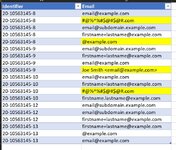
Sheet 1 has Id's and email addresses columns, Each Id has many emails, sometimes blanks too,. Each Id has multiple rows in Sheet 1.

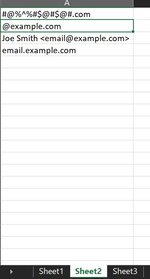
Sheet 2 has list of keywords words to use as exclude lists for email addresses.

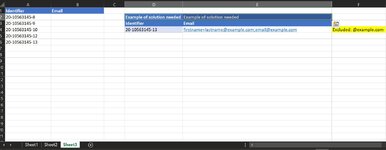
Sheet 3 has Id's, and Email addresses columns. Each Id is a unique row in Sheet 3.

I need to match Id's in sheet 3 to Id's in Sheet 1, get a list of unique, non blanks email addresses from sheet 1, filter out email addresses based on the sheet 2 exclude list keywords(partial matches), and concatenate all the emails (that are not partially matching the exclude list) with a concatenation operation like semi colon or comma.

I am not that good with array formula. I need to work on it, and many other things in excel.

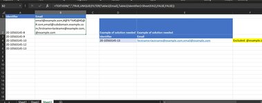
This rudimentary formula I have constructed identifies the ID from sheet 3 to all rows with the same ID in Sheet 1, gets the email addresses and concatenates them with a comma operator

=TEXTJOIN(",",TRUE,UNIQUE(FILTER(Table1[Email],Table1[Identifier]=Sheet3!A2),FALSE,FALSE))

I have not been able to progress on it despite many hours of trial and error. I would appreciate any help I can receive on it.

Thank you, everyone !
 

Attachments

  • Sheet 3 sample.JPG
    Sheet 3 sample.JPG
    128.8 KB · Views: 21
  • sheet 2 sample.JPG
    sheet 2 sample.JPG
    37 KB · Views: 21
  • Sheet1-sample.JPG
    Sheet1-sample.JPG
    127.9 KB · Views: 22
  • Formula-Sheet3 sample.JPG
    Formula-Sheet3 sample.JPG
    152.9 KB · Views: 23

Excel Facts

Last used cell?
Press Ctrl+End to move to what Excel thinks is the last used cell.
Here is one approach. You will see I converted the two tables to formal Excel tables (using Ctrl-t), with the table on Sheet1 being called Table1 and the exclusion table on Sheet2 being called Table2.
Cell Formulas
RangeFormula
A2:A6A2=UNIQUE(Table1[Identifier])
B2:B6B2=TEXTJOIN("; ",TRUE,UNIQUE(FILTER(FILTER(Table1[Email],Table1[Identifier]=A2,""), NOT(ISNUMBER(XMATCH(FILTER(Table1[Email],Table1[Identifier]=A2,""),Table2[Exclude List]))))))
Dynamic array formulas.

To facilitate further help, here are the source sheets used from XL2BB:
Book2
AB
1IdentifierEmail
220-10563145-8email@example.com
320-10563145-8#%^.com
420-10563145-8email@subdomain.example.com
520-10563145-8firstname+lastname@example.com
620-10563145-8@example.com
720-10563145-9email@subdomain.example.com
820-10563145-9firstname+lastname@example.com
920-10563145-9email@example.com
1020-10563145-9Joe Smith <email@example.com>
1120-10563145-10email@example.com
1220-10563145-10firstname+lastname@example.com
1320-10563145-10#%^.com
1420-10563145-10firstname.lastname@example.com
1520-10563145-12email@subdomain.example.com
1620-10563145-12firstname+lastname@example.com
1720-10563145-12firstname+lastname@example.com
1820-10563145-13firstname+lastname@example.com
1920-10563145-13@example.com
2020-10563145-13email@example.com
Sheet1

Book2
A
1Exclude List
2#%^.com
3@example.com
4Joe Smith <email@example.com>
5email.example.com
Sheet2
 
Last edited:
Upvote 0
Solution
Here is another version, shortened with the LET function and forming the exclusion list differently:
Cell Formulas
RangeFormula
A2:A6A2=UNIQUE(Table1[Identifier])
B2:B6B2=LET(flist,FILTER(Table1[Email],Table1[Identifier]=A2,""),TEXTJOIN("; ",TRUE,UNIQUE(FILTER(flist,NOT(COUNTIF(Table2[Exclude List],flist))))))
Dynamic array formulas.
 
Upvote 0
Hi Kirk,

I am getting #CALC! error, by the way the ID's in Sheet 3 are hyperlinked ID's, just an FYI. Let me check and get back to you on this. I got pulled away into time sucking support requests and just could not even write back here.

in ID COlumn of Sheet 3 this formula is present
=HYPERLINK(CONCATENATE("#'SHEET 1'!A",MATCH("<ID NAME>",'SHEET 1'!A:A,0)),"ID NAME")
 
Upvote 0
Hello Kirk,

Thank you for your help and solutions, I think your formula needs a very small adjustment to accomodate for the cases when the exclude list matches the emails found by your first solution.

=TEXTJOIN("; ",TRUE,UNIQUE(FILTER(FILTER(Table1,Table1[Identifier]=A2,""), NOT(ISNUMBER(XMATCH(FILTER(Table1[Email],Table1[Identifier]=A2,""),Table2[Exclude List]))))))

=TEXTJOIN("; ",TRUE,UNIQUE(FILTER(FILTER(Table1[Email],Table1[Identifier]=A2,""), NOT(ISNUMBER(XMATCH(FILTER(Table1[Email],Table1[Identifier]=A2,""),Table2[Exclude List])))[COLOR=rgb(250, 197, 28)],"BLANK"[/COLOR])))

This will accommodate for blank values and prevent dynamic array formulas from throwing a #CALC! error when the filter is left with a blank array, in those cases where you try to match the emails you have against an exclude list, and you find that the emails are to be excluded due to match with the exclude list. In this situation Filter is unable to deal with a empty array and throws this error.

For Reference:
https://exceljet.net/formula/how-to-fix-the-calc-error
 
Upvote 0
Thanks for the feedback and commentary. Regarding the #CALC! error, I didn't see any indication that there would be blanks in the data set, but if there are, wouldn't filtering them out when forming the new list in the Identifier column on Sheet3 resolve that issue? Here are both approaches mentioned earlier, modified to do this, and using the following Tablle1 and Table2 which have been modified to include blanks.

Various combinations of blanks introduced in both columns and a new "email" added to the list.
MrExcel20220327b.xlsx
AB
1IdentifierEmail
220-10563145-8email@example.com
320-10563145-8#%^.com
420-10563145-8email@subdomain.example.com
520-10563145-8firstname+lastname@example.com
620-10563145-8@example.com
720-10563145-9email@subdomain.example.com
820-10563145-9firstname+lastname@example.com
920-10563145-9email@example.com
1020-10563145-9Joe Smith <email@example.com>
1120-10563145-10email@example.com
1220-10563145-10firstname+lastname@example.com
1320-10563145-10#%^.com
1420-10563145-10firstname.lastname@example.com
1520-10563145-12email@subdomain.example.com
1620-10563145-12firstname+lastname@example.com
1720-10563145-12firstname+lastname@example.com
1820-10563145-13firstname+lastname@example.com
1920-10563145-13@example.com
2020-10563145-13
2120-10563145-13Made Up Name
22firstname+lastname@example.com
23
2420-10563145-13email@example.com
Sheet1

A blank inserted in the Exclude list:
MrExcel20220327b.xlsx
A
1Exclude List
2#%^.com
3@example.com
4Joe Smith <email@example.com>
5
6email.example.com
Sheet2

The original solution offered, except the: 1) initial creation of the Identifier column is filtered to eliminate blanks (which I believe was responsible for the error you encountered); and 2) the formula for creating the email list was shortened with the LET function.
Cell Formulas
RangeFormula
A2:A6A2=LET(fid,Table1[Identifier],UNIQUE(FILTER(fid,fid<>"")))
B2:B6B2=LET(fid,FILTER(Table1[Email],Table1[Identifier]=A2,""),TEXTJOIN("; ",TRUE,UNIQUE(FILTER(fid, NOT(ISNUMBER(XMATCH(fid,Table2[Exclude List])))))))
Dynamic array formulas.

The second solution offered with the same revision to the formula for the Identifier column:
Cell Formulas
RangeFormula
A2:A6A2=LET(fid,Table1[Identifier],UNIQUE(FILTER(fid,fid<>"")))
B2:B6B2=LET(flist,FILTER(Table1[Email],Table1[Identifier]=A2,""),TEXTJOIN("; ",TRUE,UNIQUE(FILTER(flist,NOT(COUNTIF(Table2[Exclude List],flist))))))
Dynamic array formulas.


Regarding this point:
by the way the ID's in Sheet 3 are hyperlinked ID's, just an FYI. Let me check and get back to you on this. I got pulled away into time sucking support requests and just could not even write back here.

in ID COlumn of Sheet 3 this formula is present
=HYPERLINK(CONCATENATE("#'SHEET 1'!A",MATCH("<ID NAME>",'SHEET 1'!A:A,0)),"ID NAME")
...I don't quite follow whether this is an issue. Are you saying that the list of email addresses shown in Sheet3 by the formulas are supposed to launch an email client if any one of them is selected?
 
Upvote 0
Hi Kirk,

I'm really sorry about my incomplete explanations,

I was rushing to complete this report.

So here goes how it looks

Sheet 1( has Id's and email addresses columns, Each Id has many emails, sometimes blanks too,. Each Id has multiple rows in Sheet 1. This is from a database into which emails were put in through a manual process, sometimes with errors and sometimes none, blanks result from it.

Sheet 2 has list of keywords words to use as exclude lists for email addresses. Excluded are incorrect email addresses.

Sheet 3 is my report and it has Id's, and Email addresses columns. Each Id is a unique row in Sheet 3. and emails from sheet1 are concatenated together to present all data in one row.

Sheet 3 ID column has another ID column duplicated(into which the ID is presented as a hyperlink to the Sheet 1, the hyperlink can point to one row of sheet 1 or a cell range

IN the second ID column(duplicate) of Sheet 3 below formula is present:
=HYPERLINK(CONCATENATE("#'Sheet1'!A",MATCH($A2,'Sheet1'!$A:$A,0),":Z",SUMPRODUCT(MAX(ROW('Sheet1'!$A:$A)*($A2='Sheet1'!$A:$A)))),$A2)

The above formula is the template I have used to lead the user from Sheet 3 to many other data Sheets for other columns(say for example Amazon buys, Walmart buys, Big box store1 buys, Big box Store2 buys etc.) similar to the email address that we started this post with. Similarly I have used your formula as a template to concatenate data and show it in other columns of Sheet 3 as just stated in the previous sentence.

I will try out your improved formula tonight and get back to you tomorrow about it.

Thank you, Kirk for being an awesome Excel mentor to me !

Best Regards.
 
Upvote 0
Thanks for the explanation. Your previous post referred to a "SHEET 1" and <ID NAME>, and I wasn't following your point. Your latest post clears that up and I see how the hyperlink works. Hopefully the filtering tweak in the formula addresses the issue you encountered...I haven't encountered any problems with blanks, but please post back if you do.
 
Upvote 0

Forum statistics

Threads
1,223,705
Messages
6,173,985
Members
452,540
Latest member
haasro02

We've detected that you are using an adblocker.

We have a great community of people providing Excel help here, but the hosting costs are enormous. You can help keep this site running by allowing ads on MrExcel.com.
Allow Ads at MrExcel

Which adblocker are you using?

Disable AdBlock

Follow these easy steps to disable AdBlock

1)Click on the icon in the browser’s toolbar.
2)Click on the icon in the browser’s toolbar.
2)Click on the "Pause on this site" option.
Go back

Disable AdBlock Plus

Follow these easy steps to disable AdBlock Plus

1)Click on the icon in the browser’s toolbar.
2)Click on the toggle to disable it for "mrexcel.com".
Go back

Disable uBlock Origin

Follow these easy steps to disable uBlock Origin

1)Click on the icon in the browser’s toolbar.
2)Click on the "Power" button.
3)Click on the "Refresh" button.
Go back

Disable uBlock

Follow these easy steps to disable uBlock

1)Click on the icon in the browser’s toolbar.
2)Click on the "Power" button.
3)Click on the "Refresh" button.
Go back
Back
Top