Mapping Fields based on neighbouring cells within a report & can it be scripted?

[nickhills1]

Ladies and Gents.. Hoping to get your expertise.

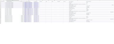
I have a report which gets generated weekly of new companies who have been added to our database. I want to import this report into a different system, but need to reformat the data to allow it to happen.
At the moment a single company's data is split across multiple rows (based on differing address fields).
I want to pull that data into a single row per company (please see the sample data in the attachment).

The second part of my question is : I will be leaving this company in a months time, but want this process to be super simple for the person replacing me. The report always comes out in the same format, although sometimes with more or less companys to be added.
Is there any way that your solution can be automated, so that when the next person opens next months report, he/she can run a script etc to reformat the data?

Many thanks in advance all

Nick

 

[Kaper]

I'm not sure if PIVOTBY function is available in Excel 2021. In Excel 365 it is , but probably in 2021 not

But If it's not, you may be able to obtain similar result with pivot table, or even better with Power Query:

While active cell in is in "Current Report" data cells Use Data->Get & transform->From Table/Range
In PQ editor select Form Question column (click on header) and use Transform->Pivot. USe Form Item as Value and in advanced options use "Do not Aggregate".
Then Close PQ editor and agree to save results.
Note that operations and cards/groups can have slightly different names as: 1) I use non-English Excel, 2) it is different Excel version

Both in Pivotby and Power Query solutions you can paste new input data over old data and have new results (in PQ it requires right click on result table (green one) and Refresh.

Zeszyt2.xlsx
	A	B	C	D	E	F	G	H	I	J	K	L	M	N
1	Company ID	Name	bla	Form Question	Form Item					City	Country	Mailing Address	Whatever
2	1	a	aaa	City	Paris		1	a	aaa	Paris	France	1 Rue de Funes	This and that
3	1	a	aaa	Country	France		2	b	bb	London	UK	10 Buckingham Rd	That and something
4	1	a	aaa	Mailing Address	1 Rue de Funes
5	1	a	aaa	Whatever	This and that
6	2	b	bb	City	London
7	2	b	bb	Country	UK
8	2	b	bb	Mailing Address	10 Buckingham Rd
9	2	b	bb	Whatever	That and something
10
Sheet1

Cell Formulas
Range	Formula
G1:M3	G1	=PIVOTBY(A:C,D:D,E:E,CONCAT,1,0,,0,,A:A<>"")
Dynamic array formulas.