Macro to hide rows with null values or blanks in all columns.

[R420]

Hi,

I have a sheet in my workbook that compiles info from 4 other sheets using formulas to call up cells from other sheets, for example: ='STEAM (SH)'!D3 . this leaves me with rows that have info in every column or just one column at times.
I want to be able to quickly hide the rows that have null values or blanks in all columns but keep the row if it has any data showing.
I tried following tutorials that used identifier columns but since my cells have formulas, it wouldn't differentiate between a cell with null data in it and a cell that is actually blank.

is there a macro that I could use that would hide/unhide all rows that are returning null values (blanks) as well as actual blank cells with no data in them in all columns but keep the rows that might have only one cell returning data. My range I am working in is A3:M100.

Thanks for your time.

 

[thirty_two]

I can update this if you need to check a range of columns instead of an entire row, but if this works, then great!

Sub HideUnhide()

Dim rng As Range
Set rng = Range("A3:M3")

For i = 1 To 98
    If Application.CountA(rng.Cells(i, 1).EntireRow) = 0 Then
        If rng.Cells(i, 1).EntireRow.Hidden Then
            rng.Cells(i, 1).EntireRow.Hidden = False
        Else
            rng.Cells(i, 1).EntireRow.Hidden = True
        End If
    End If
Next

End Sub

 

[bebo021999]

I would suggest using helper column to create autofilter on this column

Option Explicit
Sub test()
Application.ScreenUpdating = False
Dim i&, count&, rng As Range, cell As Range, helper As Range
Set rng = Range("A2:M2")
ActiveSheet.AutoFilterMode = False
Set helper = Range("N3:N100") ' or using any column that available
helper.ClearContents
    For i = 1 To (100 - 2) ' if working range was A2:M100, loop through each row
        count = 0
        For Each cell In rng.Offset(i, 0)
            count = count + Len(cell) ' sum all length of cells each row
        Next
        With helper.Cells(i)
            If count = 0 Then ' all values are blank or null: sum of length = 0
                .Value = "" ' marks row that all values are blank or null, with blank
            Else: .Value = "@" ' marks used row , with "@"
            End If
        End With
    Next
Range("N2:N100").AutoFilter ' adjust range, to include helper column
Application.ScreenUpdating = True
End Sub

Book1
	A	B	C	D	E	F	G	H	I	J	K	L	M	N
1
2
3	1													@
4		1	1	1										@
5
6							1							@
7		a	a	a										@
8
9
10
11
12
13
14
15
16
17
18				Formulla in E7, E8: =""
Sheet1

Cell Formulas
Range	Formula
E5,E7:E8	E5	=""

 

[R420]

I can update this if you need to check a range of columns instead of an entire row, but if this works, then great!

Sub HideUnhide()

Dim rng As Range
Set rng = Range("A3:M3")

For i = 1 To 98
    If Application.CountA(rng.Cells(i, 1).EntireRow) = 0 Then
        If rng.Cells(i, 1).EntireRow.Hidden Then
            rng.Cells(i, 1).EntireRow.Hidden = False
        Else
            rng.Cells(i, 1).EntireRow.Hidden = True
        End If
    End If
Next

End Sub

Thanks for the reply.

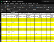
I'm pretty new to macro's and am not an Excel expert so forgive me if I'm missing something. I copied this into the visual basic window and ran the macro, nothing appeared to happen. I've attached an image of the top portion of my spreadsheet as an example. I've added data to random cells while I test this but I am trying to automatically hide all the yellow (empty) rows and since this changes I'd prefer something automated. All of these cells have formulas in them like the one shown in the image to read info from cells on other sheets.

 

[R420]

I would suggest using helper column to create autofilter on this column

Option Explicit
Sub test()
Application.ScreenUpdating = False
Dim i&, count&, rng As Range, cell As Range, helper As Range
Set rng = Range("A2:M2")
ActiveSheet.AutoFilterMode = False
Set helper = Range("N3:N100") ' or using any column that available
helper.ClearContents
    For i = 1 To (100 - 2) ' if working range was A2:M100, loop through each row
        count = 0
        For Each cell In rng.Offset(i, 0)
            count = count + Len(cell) ' sum all length of cells each row
        Next
        With helper.Cells(i)
            If count = 0 Then ' all values are blank or null: sum of length = 0
                .Value = "" ' marks row that all values are blank or null, with blank
            Else: .Value = "@" ' marks used row , with "@"
            End If
        End With
    Next
Range("N2:N100").AutoFilter ' adjust range, to include helper column
Application.ScreenUpdating = True
End Sub

Book1
	A	B	C	D	E	F	G	H	I	J	K	L	M	N
1
2
3	1													@
4		1	1	1										@
5
6							1							@
7		a	a	a										@
8
9
10
11
12
13
14
15
16
17
18				Formulla in E7, E8: =""
Sheet1

Cell Formulas
Range	Formula
E5,E7:E8	E5	=""

Thanks for the reply.

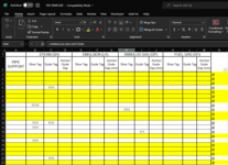
I tried this macro as well and it did mark my N column with @ symbols but it did not differentiate between empty rows and rows with data. It placed @ symbols on every row.

I am very new to using macro's in Excel so if there are things you are assuming I know, then I assure you I do not haha