LET function and income stream table

[Holger]

Hi there,

I want to update some spreadsheets with more modern formulas like the LET function. The task is to use the LET function to create a table that shows an income stream (=monthly withdrawals) from a savings account that earns interest. In the past I used endless formulas to create each col of the table.

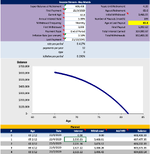
Screen1 shows at the top input data (still needs removal of unnecessary fields) and at the bottom the old table.

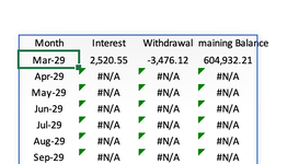
Screen 2 is the new table I would like to create with the LET function. As you can see, first two works but rest not. Current LET function I use is as follows:
=LET(
openbal,E4,
annualrate,E7,
periodrate,annualrate/12,
pv,-openbal,
inflat,E16,
monthpers, EDATE(E5,SEQUENCE(H7,1,0)),
withdrawpmts,(1+inflat)*H6,
bals,SCAN(openbal,withdrawpmts,LAMBDA(x,r,x-r)),
intearnt, bals*periodrate,
VSTACK(
HSTACK("Month","Interest","Withdrawal","Remaining Balance"),
HSTACK(monthpers,intearnt,-withdrawpmts,balls)
))
For info, interest is previous period balance multiplied with monthly interest rate, while withdrawal is previous withdrawal multiplied with monthly inflation. I think what I cant work out is how to move forwardperiod by period. I managed to get the periods into the first column but rest does not work.
I'm clearly making some mistakes here so any help would be greatly appreciated.

Cheers everyone

 

[StephenCrump]

I think this is what you're trying to do - running the balance down to nil?

It's a little convoluted, because with an inflation assumption we can't use the standard Excel financial functions.

	A	B	C	D
1	Start	21 Mar 2029
2	Balance	608,408.33
3	N	24
4		p.a.	p.m.
5	Return	5.0%	0.417%
6	Inflation	3.5%	0.292%
7
8	Date	Interest	Payment	Balance
9	21 Mar 2029			608,408.33
10	21 Apr 2029	2,535.03	25,822.28	585,121.09
11	21 May 2029	2,438.00	25,897.59	561,661.50
12	21 Jun 2029	2,340.26	25,973.13	538,028.63
13	21 Jul 2029	2,241.79	26,048.88	514,221.54
14	21 Aug 2029	2,142.59	26,124.86	490,239.27
15	21 Sep 2029	2,042.66	26,201.05	466,080.88
16	21 Oct 2029	1,942.00	26,277.47	441,745.41
17	21 Nov 2029	1,840.61	26,354.12	417,231.90
18	21 Dec 2029	1,738.47	26,430.98	392,539.38
19	21 Jan 2030	1,635.58	26,508.07	367,666.89
20	21 Feb 2030	1,531.95	26,585.39	342,613.45
21	21 Mar 2030	1,427.56	26,662.93	317,378.08
22	21 Apr 2030	1,322.41	26,740.70	291,959.79
23	21 May 2030	1,216.50	26,818.69	266,357.60
24	21 Jun 2030	1,109.82	26,896.91	240,570.51
25	21 Jul 2030	1,002.38	26,975.36	214,597.53
26	21 Aug 2030	894.16	27,054.04	188,437.65
27	21 Sep 2030	785.16	27,132.95	162,089.86
28	21 Oct 2030	675.37	27,212.08	135,553.15
29	21 Nov 2030	564.80	27,291.45	108,826.50
30	21 Dec 2030	453.44	27,371.05	81,908.89
31	21 Jan 2031	341.29	27,450.88	54,799.30
32	21 Feb 2031	228.33	27,530.95	27,496.68
33	21 Mar 2031	114.57	27,611.25	0.00
34
Sheet1

Cell Formulas
Range	Formula
C5:C6	C5	=B5/12
A8:D33	A8	=LET(s,SEQUENCE(N),p,PMT((1+ret)/(1+inf)-1,N,-Balance)*(1+inf)^s,bal,VSTACK(Balance,Balance*(1+ret)^s-SCAN(0,p,LAMBDA(a,b,a*(1+ret)+b))),VSTACK({"Date","Interest","Payment","Balance"},HSTACK(Start,"","",Balance),HSTACK(EDATE(Start,s),DROP(ret*bal,-1),p,DROP(bal,1))))
Dynamic array formulas.

Named Ranges
Name	Refers To	Cells
Balance	=Sheet5!$B$2	A8
inf	=Sheet5!$C$6	A8
N	=Sheet5!$B$3	A8
ret	=Sheet5!$C$5	A8
Start	=Sheet5!$B$1	A8

I've shown a small example (only 24 months) to fit on screen better. How do you calculate your initial withdrawal of 3,466.01? I get ...

Start	21 Mar 2029
Balance	608,408.33
N	199
	p.a.	p.m.
Return	5.0%	0.417%
Inflation	3.5%	0.292%
Date	Interest	Payment	Balance
21 Mar 2029			608,408.33
21 Apr 2029	2,535.03	3,464.10	607,479.26
21 May 2029	2,531.16	3,474.21	606,536.22
21 Jun 2029	2,527.23	3,484.34	605,579.11
21 Jul 2029	2,523.25	3,494.50	604,607.85
.....
21 Jul 2045	101.27	6,112.75	18,292.62
21 Aug 2045	76.22	6,130.58	12,238.27
21 Sep 2045	50.99	6,148.46	6,140.80
21 Oct 2045	25.59	6,166.39	0.00

 

[Holger]

Hi Stephen,

thanks very much for your assistance. I meanwhile worked out the interest column but not yet the withdrawal. Your above solution works great with 2 mods I would like to ask:

1. The initial withdrawal should be a simple input field, that I enter a $ value.
2. The withdrawals and interest should stop, once the remaining balance is 0

Again much appreciated your help.

Cheers H

 

[StephenCrump]

How about:

	A	B	C	D
1	Start	21 Mar 2029
2	Balance	100,000.00
3	Payment	4,000.00
4	N	26
5		p.a.	p.m.
6	Return	5.0%	0.417%
7	Inflation	3.5%	0.292%
8
9	Date	Interest	Payment	Balance
10	21 Mar 2029			100,000.00
11	21 Apr 2029	416.67	4,000.00	96,416.67
12	21 May 2029	401.74	4,011.67	92,806.74
13	21 Jun 2029	386.69	4,023.37	89,170.06
14	21 Jul 2029	371.54	4,035.10	85,506.50
15	21 Aug 2029	356.28	4,046.87	81,815.91
16	21 Sep 2029	340.90	4,058.67	78,098.13
17	21 Oct 2029	325.41	4,070.51	74,353.03
18	21 Nov 2029	309.80	4,082.38	70,580.45
19	21 Dec 2029	294.09	4,094.29	66,780.24
20	21 Jan 2030	278.25	4,106.23	62,952.26
21	21 Feb 2030	262.30	4,118.21	59,096.35
22	21 Mar 2030	246.23	4,130.22	55,212.37
23	21 Apr 2030	230.05	4,142.27	51,300.15
24	21 May 2030	213.75	4,154.35	47,359.55
25	21 Jun 2030	197.33	4,166.47	43,390.42
26	21 Jul 2030	180.79	4,178.62	39,392.59
27	21 Aug 2030	164.14	4,190.81	35,365.92
28	21 Sep 2030	147.36	4,203.03	31,310.25
29	21 Oct 2030	130.46	4,215.29	27,225.42
30	21 Nov 2030	113.44	4,227.58	23,111.28
31	21 Dec 2030	96.30	4,239.91	18,967.66
32	21 Jan 2031	79.03	4,252.28	14,794.41
33	21 Feb 2031	61.64	4,264.68	10,591.37
34	21 Mar 2031	44.13	4,277.12	6,358.38
35	21 Apr 2031	26.49	4,289.60	2,095.28
36	21 May 2031	8.73	4,302.11	-2,198.09
37
Sheet1

Cell Formulas
Range	Formula
B4	B4	=ROUNDUP(NPER((1+ret)/(1+inf)-1,payment/(1+inf),-Balance),0)
C6:C7	C6	=B6/12
A9:D36	A9	=LET(s,SEQUENCE(N),p,payment*(1+inf)^(s-1),bal,VSTACK(Balance,Balance*(1+ret)^s-SCAN(0,p,LAMBDA(a,b,a*(1+ret)+b))),VSTACK({"Date","Interest","Payment","Balance"},HSTACK(Start,"","",Balance),HSTACK(EDATE(Start,s),DROP(ret*bal,-1),p,DROP(bal,1))))
Dynamic array formulas.

Named Ranges
Name	Refers To	Cells
Balance	=Sheet5!$B$2	B4, A9
inf	=Sheet5!$C$7	B4, A9
N	=Sheet5!$B$4	A9
payment	=Sheet5!$B$3	B4, A9
ret	=Sheet5!$C$6	B4, A9
Start	=Sheet5!$B$1	A9

 

[Holger]

Hi Stephen, thank you so much. I was able to copy it into my file, named the ranges and voila, it is working perfectly. One major area I missed was, that I could enquiry about # of period with NPER formula.

Awesome help, thanks very much again.

 

[Holger]

Stephen, in the 1st Hstack formula I replaced your “” with 0 as I use the resulting array later on in other formulas, which gave me #value errors. Once replaced those work as well.

Thanks again.

 

[StephenCrump]

You're welcome. I'm glad it's all working for you.