Last Attempt for HELP on this problem

[thhynes]

So this is my last attempt to solve this problem - hoping that I can have some guidance

Requests for examples of the data I have had to be created as all of the
data I have is proprietary and protected by state and federal rules so I can't share the real data I have tried my best to show
what the data looks like in this example

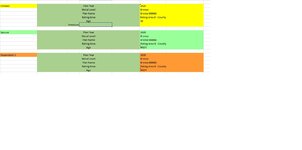
USER END SHEET - where the representative enters the relevant information

BASED on the following information

Plan Year Selection - either 2020 or 2021
Metal Level - Catastrophic, Bronze, Silver, Gold
Plan Name - Bronze - AAAA, Bonze BBBB, or Bronze CCCC
Rating Area by Name
Rating Area by Number
AGE
.....> FILL a CELL with the correct Premium - based on the information entered from the USER DATA SHEET

NOTE the Spreadsheet does not show this however
There is (ONE) Catastrophic Plan
There are (FOUR) Bronze Level Plans
There is (ONE) Silver
There are (THREE) Gold
9 Plans all together

3 Sheets Created in ONE workbook

User Entry Sheet
Calculation Sheet - Created this to keep things in check for logical and organizational reasons
Data Table
Although Separate here I can include it on the Calculation Sheet as well


I have attempted the following formulas with each one failing

=VLOOKUP(E6,'[Validations Working.xlsx]#Data Validation Work Sheet (2)'!$AD$150:$AJ$7493,7,FALSE) ( my formula from the official workbook I am creating not valid to example)

=INDEX(A1:h7493,MATCH(CELL,Cell:Cell)*(CELL,Cell:CELL)*(Cell,Cell:CELL)0,"""Premium Column) --- return this value to the appropriate cell on
the Calculation Sheet.... then make the Appropriate Cell on the User End Sheet = this VALUE

This is the LAST STEP and I can't figure it out

Find attached a represenative excell workbook with all three sheets

Thank you

 

[thhynes]

This is the DATA sheet for the problem above

 

[thhynes]

Data Sheet

 

[thhynes]

 

[smozgur]

MrExcel has a tool called “XL2BB” that lets you post samples of your data that will allow us to copy/paste it to our Excel spreadsheets, so we can work with the same copy of data that you are. Instructions on using this tool can be found here: XL2BB Add-in

Note that there is also a "Test Here” forum on this board. This is a place where you can test using this tool (or any other posting techniques that you want to test) before trying to use those tools in your actual posts.