Issues using FILTER formula

[crismat09]

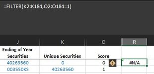
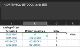
I am trying to use the FILTER formula to return only the results that meet a criteria listed on column B. On column A, I am using the UNIQUE function to bring unique values from a different table. Column B has 1/0 values related to the data on column A. In column C, I would like to have only the values in column A that have Yes in column B. For this I am using the formula:

=FILTER(A2:A184,B2:B184 =1)

However, the result of the formula is #n/a

Any idea on how to fix the issue?

Additional details:
Columns ABC are not in a table but in range format
When selecting the array for the filter formula by using crtl+shift+down, the range returned is "A2#". I needed to manually update the array to reflect A2:A184
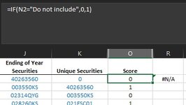
The values on column B (1/0) are not typed numbers, the result of an IF formula.

 

[Alex Blakenburg]

You are mixing and matching the column references eg images use different columns than your narration.
I am going to run with your image references.

The only way that I can replicate that behaviour is if your column N is also a formula and is returning #N/A which causes your IF statement in Column N to return #N/A.
This in turn is causing the filter to return #N/A.
(Note: N/A in columns I to K do not seem to cause the issue)
I suggest you wrap whatever formula you have in Column N in an if error function.

Book1
	I	J	K	L	M	N	O	P	Q	R
1	Col I	Col J	Unique			Criteria	Score			Result
2	10	0	0			Do not include	0			#N/A
3	20	20	10				1
4	30	40	20			Do not include	0
5	40	60	30				1
6	50	80	40			Do not include	0
7	60	100	50				1
8			60			Do not include	0
9			80			#N/A	#N/A
10			100			Do not include	0
Sheet1

Cell Formulas
Range	Formula
K2:K10	K2	=SORT(UNIQUE(TOCOL(I2:J7)))
R2	R2	=FILTER(K2:K184,O2:O184=1)
I3:I7	I3	=I2+10
J3:J7	J3	=J2+20
N9	N9	=NA()
O2:O10	O2	=IF(N2="Do not include",0,1)
Dynamic array formulas.