Index Match with zeros and duplicate data.

[Bob_ipc]

Hey all, Thanks for taking the time to review my question. I must be missing something simple but for whatever reason I am missing something.
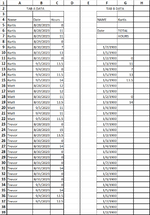
In "Tab A" I have a list of "A" names, "B" dates and "C" total hours, In "Tab B" I have "A9:A39" each date of the selected month, "A1" the name I want to look up and "B9:B39" is where I would like the total hours to feed into based on the date and name.

Currently in "H9" I have =IFERROR(XLOOKUP(1,('TAB A'!A$5:A$39='TAB B'!G$4)*('TAB A'!B$5:B$39='TAB B'!F9),'TAB A'!C$9:D$39),"")

However there are some duplicate dates in "TAB A" Column B with corresponding data in Column "C" that I would like in "TAB B" Column "G" the formula that I have only takes the first line of data that it sees and ignores the data below it.

How can I get the SUM of Data in "TAB B" Column "G" based on the Name and Date from "TAB A"? I am sure I am missing something simple but my brain block is not letting me get through this, Any help would be really appriciated.

Thanks

 

[Fluff]

I suggest that you update your Account details (or click your user name at the top right of the forum) so helpers always know what Excel version(s) & platform(s) you are using as the best solution often varies by version. (Don’t forget to scroll down & ‘Save’)

You need to use the SUMIFS function. SUMIFS Function

 

[Bob_ipc]

Hey Fluff,

Thanks for the reply, I have updated my account details thank you. Also I have tried SUMIFS as well and I get the same results for some reason?

 

[Fluff]

What was the sumifs formula you tried?

 

[Bob_ipc]

I "Tab B" Cell "H9" I put =SUMIFS(tab a!C$5:C$39,tab a!B$5:B$39,tab b!G$4,tab a!B$5:B$39,tab a!F9)

 

[Fluff]

That looks as though the 1st B5:B39 should be col A instead.

 

[Bob_ipc]

Yep that did it, Duh I knew I just had a stupid blockage in my head haha.

Thank you Fluff

 

[Fluff]

Glad to help & thanks for the feedback