Index Match multiple results skip the blanks

[rdbauer83]

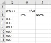
Hi there hope someone can help as I am about to lose it because I know there is something simple. I have a table and I need another sheet to return only cells that match 2 given criteria and aren't empty. I have 2 worksheets and need the information from worksheet 2 to show up on worksheet 1 with given criteria and only cells from worksheet 2 that have information. I have uploaded worksheet 1 without the info, worksheet 2 that has the information needed, and final result which is what I need worksheet 1 to look like. Thank you all for the help!

 

[Peter_SSs]

Welcome to the MrExcel board!

For the future, please consider the following so that we can easily copy/paste your sample data to test with as most helpers are not that keen on manually typing sample data.
MrExcel has a tool called “XL2BB” that lets you post samples of your data that will allow us to copy/paste it to our Excel spreadsheets, so we can work with the same copy of data that you are. Instructions on using this tool can be found here: XL2BB Add-in

Note that there is also a "Test Here” forum on this board. This is a place where you can test using this tool (or any other posting techniques that you want to test) before trying to use those tools in your actual posts.

Assuming the values in R2 of Sheet1 and row 4 of Sheet2 are actual dates (formatted to show month/day only) then with Microsoft 365 (or 2021) try this.

rdbauer83.xlsm
	B	C	D	E	F	G	H	I	J
4			4/25	4/26	4/27	4/28	4/29	4/30	5/1
5
6	HELP	Name 1	a	b	c	d
7	HELP	Name 2				e	f	g	h
8	HELP	Name 3	i				j	k	l
9	HELP	Name 4	m	n	o	p	q	r	s
10	HELP	Name 5
Sheet2

rdbauer83.xlsm
	Q	R	S
2		4/28
3		TIME	NAME
4
5
6
7	HELP	d	Name 1
8	HELP	e	Name 2
9	HELP	p	Name 4
10
Sheet1

Cell Formulas
Range	Formula
Q7:S9	Q7	=LET(col,INDEX(Sheet2!D6:J10,0,MATCH(R2,Sheet2!D4:J4,0)),FILTER(CHOOSE({1,2,3},Sheet2!B6:B10,col,Sheet2!C6:C10),col<>""))
Dynamic array formulas.

 

[rdbauer83]

Thank you for the reply. I apologize for the formatting as this is the first time I have posted on a board. That did do what I wanted, now I have different categories and have a different number of people for each on any given day with different times. With that, what is a solution for this? Thank you again
Sheet 1

Book1
	Q	R	S
2		4/28
3		TIME	NAME
4
5
6
7	HELP
8	HELP
9	HELP
10	HELP
11	HELP
12	ALPHA
13	ALPHA
14	ALPHA
15	ALPHA
16	ALPHA
17	BRAVO
18	BRAVO
19	BRAVO
20	BRAVO
21	BRAVO
Sheet1

Sheet 2

Book1
	B	C	D	E	F	G	H	I	J
4			4/25	4/26	4/27	4/28	4/29	4/30	5/1
5
6	HELP	Name 1	a	b	c	d
7	HELP	Name 2				e	f	g	h
8	HELP	Name 3	i				j	k	l
9	HELP	Name 4	m	n	o	p	q	r	s
10	HELP	Name 5		t	u	v
11	ALPHA	Name 6	w				x	y	z
12	ALPHA	Name 7		A	B	C		D
13	ALPHA	Name 8	E	F		G		H
14	ALPHA	Name 9	I		J		K		L
15	ALPHA	Name 10				M	N	O	P
16	ALPHA	Name 11	Q	R	S		T
17	ALPHA	Name 12		U	V		W		X
18	ALPHA	Name 13	Y	Z	AA	BB
19	BRAVO	Name 18	CC	DD	EE	FF
20	BRAVO	Name 19				GG	HH	II	JJ
21	BRAVO	Name 20	KK	LL			MM	NN
22	BRAVO	Name 21	OO				PP	QQ	RR
23	BRAVO	Name 22		SS	TT	UU			VV
24	BRAVO	Name 23	WW	XX	YY	ZZ
25	BRAVO	Name 24				AAA	BBB	CCC	DDD
26	BRAVO	Name 25	EEE	FFF			GGG	HHH
27	BRAVO	Name 26			III	JJJ	LLL
Sheet2

Final sheet 1 date 4/28

Book1
	Q	R	S
2		4/28
3		TIME	NAME
4
5
6
7	HELP	d	Name 1
8	HELP	e	Name 2
9	HELP	p	Name 4
10	HELP	v	Name 5
11	HELP	blank	blank
12	ALPHA	C	Name 7
13	ALPHA	G	Name 8
14	ALPHA	M	Name 10
15	ALPHA	BB	Name 13
16	ALPHA	blank	blank
17	BRAVO	FF	Name 18
18	BRAVO	GG	Name 19
19	BRAVO	UU	Name 22
20	BRAVO	ZZ	Name 23
21	BRAVO	AAA	Name 24
22	BRAVO	JJJ	Name 26
23	BRAVO	blank	blank
24	BRAVO	blank	blank
Sheet1

Final if date in Sheet1!R2=4/27

Book1
	Q	R	S
2		4/27
3		TIME	NAME
4
5
6
7	HELP	c	Name 1
8	HELP	o	Name 4
9	HELP	u	Name 5
10	HELP	blank	blank
11	HELP	blank	blank
12	ALPHA	B	Name 7
13	ALPHA	JJJ	Name 9
14	ALPHA	S	Name 11
15	ALPHA	V	Name 12
16	ALPHA	AA	Name 13
17	BRAVO	EE	Name 18
18	BRAVO	TT	Name 22
19	BRAVO	YY	Name 23
20	BRAVO	III	Name 26
21	BRAVO	blank	blank
22	BRAVO	blank	blank
23	BRAVO	blank	blank
24	BRAVO	blank	blank
Sheet1

 

[Peter_SSs]

I don't understand the logic.

For 4/28
For HELP original data has 1 blank row and your expected results has 1 blank row.
For ALPHA original data has 4 blank rows and expected results has 1 blank row.
For BRAVO original data has 3 blank rows and expected results has 2 blank rows.

 

[rdbauer83]

I don't understand the logic.

For 4/28
For HELP original data has 1 blank row and your expected results has 1 blank row.
For ALPHA original data has 4 blank rows and expected results has 1 blank row.
For BRAVO original data has 3 blank rows and expected results has 2 blank rows.

Sorry, maybe this helps, "Sheet 2" is an overall total staffing sheet with names and shifts that each person will be working for that week. "Sheet 1" is a daily staffing sheet where we won't have every person working everyday in that area but based on the day of the week we will need different levels of staff to work. "HELP", "ALPHA", AND "BRAVO" are the positions, names (self explanatory), and the letters are the shift for that date they will work. On Sheet 1 (depending on the day of the week) we will have a MAX of 5 "HELP", 5 "ALPHA", and 8 "BRAVO" workers, but on a different day we may only need 3-4. This is the first step in a workbook that has many more after and I have steps 2-20 done...I just can't get this first step to work giving me the information needed without typing in each name/shift each day or having to create another worksheet to copy and paste each day to pull data from using vlookups. Sorry hope this helps explain what it is used for

 

[Peter_SSs]

we will have a MAX of 5 "HELP", 5 "ALPHA", and 8 "BRAVO" workers,

Does that mean that Q7:Q24 in Sheet1 is already filled in with those values and your request is for formulas to fill R7:S24 only?

 

[rdbauer83]

Does that mean that Q7:Q24 in Sheet1 is already filled in with those values and your request is for formulas to fill R7:S24 only?

yes sir that is correct. Column Q has the max number of people per area that would work in a day. I just need the name and times for each area on a given day. Actually there are 90 rows in columns Q-S with possible people to fill 11 different positions on a day, but if I can get this to work then I can transpose to the rest of the sheet

 

[Peter_SSs]

yes sir that is correct.

OK, for the setup from post #3 here is my Sheet1

rdbauer83_1.xlsm
	Q	R	S
1
2		4/28
3		TIME	NAME
4
5
6
7	HELP	d	Name 1
8	HELP	e	Name 2
9	HELP	p	Name 4
10	HELP	v	Name 5
11	HELP
12	ALPHA	C	Name 7
13	ALPHA	G	Name 8
14	ALPHA	M	Name 10
15	ALPHA	BB	Name 13
16	ALPHA
17	BRAVO	FF	Name 18
18	BRAVO	GG	Name 19
19	BRAVO	UU	Name 22
20	BRAVO	ZZ	Name 23
21	BRAVO	AAA	Name 24
22	BRAVO	JJJ	Name 26
23	BRAVO
24	BRAVO
Sheet1

Cell Formulas
Range	Formula
R17:S22,R12:S15,R11,R16,R23:R24,R7:S10	R7	=LET(col,INDEX(Sheet2!D$6:J$27,0,MATCH(R$2,Sheet2!D$4:J$4,0)),IFERROR(INDEX(FILTER(CHOOSE({1,2},col,Sheet2!C$6:C$27),(col<>"")*(Sheet2!B$6:B$27=Q7)),COUNTIF(Q$7:Q7,Q7)),""))
Dynamic array formulas.

 

[rdbauer83]

OK, for the setup from post #3 here is my Sheet1

rdbauer83_1.xlsm
	Q	R	S
1
2		4/28
3		TIME	NAME
4
5
6
7	HELP	d	Name 1
8	HELP	e	Name 2
9	HELP	p	Name 4
10	HELP	v	Name 5
11	HELP
12	ALPHA	C	Name 7
13	ALPHA	G	Name 8
14	ALPHA	M	Name 10
15	ALPHA	BB	Name 13
16	ALPHA
17	BRAVO	FF	Name 18
18	BRAVO	GG	Name 19
19	BRAVO	UU	Name 22
20	BRAVO	ZZ	Name 23
21	BRAVO	AAA	Name 24
22	BRAVO	JJJ	Name 26
23	BRAVO
24	BRAVO
Sheet1

Cell Formulas
Range	Formula
R17:S22,R12:S15,R11,R16,R23:R24,R7:S10	R7	=LET(col,INDEX(Sheet2!D$6:J$27,0,MATCH(R$2,Sheet2!D$4:J$4,0)),IFERROR(INDEX(FILTER(CHOOSE({1,2},col,Sheet2!C$6:C$27),(col<>"")*(Sheet2!B$6:B$27=Q7)),COUNTIF(Q$7:Q7,Q7)),""))
Dynamic array formulas.

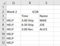
Yes that is what I needed...except on some of the rows the name is appearing below the time instead of in column "S". When I change the date some will be correct and others will not

 

[Peter_SSs]

Could we have a small sample data where that is the case so that I can investigate?