Hello! I have a set of month dates across a row and values filled in below for the months when activity occurs, blank when no activity occurs.
I need to look across multiple year spans and create a table to give me each date with a value in a nice little compact view. I've spent a couple of hours trying different solutions and reading other posts and I am ready to admit that I'm not going to be able to self serve! I get it to sorta work in a basic sample but not with real-life data. I don't understand it well enough to find where it is going wrong.
Examples below-
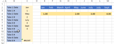
Works in theory to give me the first month and first value, second month and second value etc. However I think it just "happens" to work based on the sample data values I chose, not because the formulas are correct.

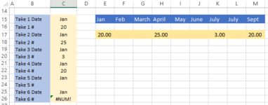
Tried with more realistic values below and it does not like my date formula. I guess I don't understand the -1, -2, etc piece. I thought it was telling it to go to the next non-blank... But it finds January as the answer every time.

The only other issue I have is why take #5 & #6 = #NUM error. Is it because there isn't a 5th or 6th value? It's saying it can't find a # but the IFNA part doesn't work because the error isn't NA????
Greatly appreciate any help and advice this group can give!
-S
I need to look across multiple year spans and create a table to give me each date with a value in a nice little compact view. I've spent a couple of hours trying different solutions and reading other posts and I am ready to admit that I'm not going to be able to self serve! I get it to sorta work in a basic sample but not with real-life data. I don't understand it well enough to find where it is going wrong.
Examples below-
Works in theory to give me the first month and first value, second month and second value etc. However I think it just "happens" to work based on the sample data values I chose, not because the formulas are correct.
Date formula- =IFNA(INDEX(E2:M2,MATCH(TRUE,INDEX(E4:M4>0,0),0)),"")
second date becomes =IFNA(INDEX(E2:M2,MATCH(TRUE,INDEX(E4:M4-1>0,0),0)),"") with increasing the subtraction part in red for each date field.
Value # formula- =IFNA(INDEX(E4:Q4,SMALL(IF(E4:Q4<>"",COLUMN(E4:Q4)-COLUMN(E4)+1),1)),"")
second value 3 becomes =IFNA(INDEX(E4:Q4,SMALL(IF(E4:Q4<>"",COLUMN(E4:Q4)-COLUMN(E4)+1),2)),"") with increasing the last # in red for each # field
Tried with more realistic values below and it does not like my date formula. I guess I don't understand the -1, -2, etc piece. I thought it was telling it to go to the next non-blank... But it finds January as the answer every time.
The only other issue I have is why take #5 & #6 = #NUM error. Is it because there isn't a 5th or 6th value? It's saying it can't find a # but the IFNA part doesn't work because the error isn't NA????
Greatly appreciate any help and advice this group can give!
-S


