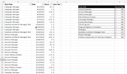
If a value of a range in column B equals a range of values in column J, then multiply F by K and fill Column G

[mcjohnson3211]

Here is my example. I'm trying to fill in column G. I hope this makes sense.

Team Role	Date	Hours	Hour Fee
Campaign Manager	8/1/2023​	0.5​	$-			Team Role	Hourly Rate
Campaign Manager	8/2/2023​	3​	$-			Account Director	$185​
Campaign Manager	8/3/2023​	1.25​	$-			Account Manager	$150​
Campaign Manager	8/3/2023​	2​	$-			Delivery Manager	$175​
Campaign Manager	8/4/2023​	1.5​	$-			Client Delivery Analyst	$150​
Campaign Manager	8/7/2023​	0.75​	$-			Campaign Manager	$100​
Campaign Manager	8/8/2023​	1.5​	$-			Content Developer	$100​
Solutions Architect/ Manager/ BSA	8/10/2023​	1​	$-			Client Engineer	$200​
Campaign Manager	8/10/2023​	1​	$-			Program Engineer/ Developer	$200​
Campaign Manager	8/14/2023​	1.5​	$-			Strategist	$200​
Solutions Architect/ Manager/ BSA	8/16/2023​	0.5​	$-			Solutions Architect/ Manager/ BSA	$175​
Delivery Manager	8/17/2023​	2.25​	$-			Project Manager	$175​
Solutions Architect/ Manager/ BSA	8/17/2023​	0.25​	$-			Creative (Copywriter, Art Director, Designer)	$185​
Delivery Manager	8/18/2023​	4​	$-
Account Manager	8/21/2023​	0.5​	$-
Account Manager	8/21/2023​	0.5​	$-
Account Manager	8/21/2023​	1​	$-
Account Director	8/21/2023​	2.25​	$-
Delivery Manager	8/21/2023​	3​	$-
Client Delivery Analyst	8/21/2023​	1.75​	$-
Account Manager	8/22/2023​	1​	$-
Account Manager	8/22/2023​	0.5​	$-
Account Director	8/22/2023​	1.5​	$-
Delivery Manager	8/22/2023​	3​	$-
Client Delivery Analyst	8/22/2023​	1.25​	$-
Delivery Manager	8/23/2023​	3​	$-
Campaign Manager	8/23/2023​	1​	$-

 

[mcjohnson3211]

Here is my example. I'm trying to fill in column G. I hope this makes sense.

Team Role	Date	Hours	Hour Fee
Campaign Manager	8/1/2023​	0.5​	$-			Team Role	Hourly Rate
Campaign Manager	8/2/2023​	3​	$-			Account Director	$185​
Campaign Manager	8/3/2023​	1.25​	$-			Account Manager	$150​
Campaign Manager	8/3/2023​	2​	$-			Delivery Manager	$175​
Campaign Manager	8/4/2023​	1.5​	$-			Client Delivery Analyst	$150​
Campaign Manager	8/7/2023​	0.75​	$-			Campaign Manager	$100​
Campaign Manager	8/8/2023​	1.5​	$-			Content Developer	$100​
Solutions Architect/ Manager/ BSA	8/10/2023​	1​	$-			Client Engineer	$200​
Campaign Manager	8/10/2023​	1​	$-			Program Engineer/ Developer	$200​
Campaign Manager	8/14/2023​	1.5​	$-			Strategist	$200​
Solutions Architect/ Manager/ BSA	8/16/2023​	0.5​	$-			Solutions Architect/ Manager/ BSA	$175​
Delivery Manager	8/17/2023​	2.25​	$-			Project Manager	$175​
Solutions Architect/ Manager/ BSA	8/17/2023​	0.25​	$-			Creative (Copywriter, Art Director, Designer)	$185​
Delivery Manager	8/18/2023​	4​	$-
Account Manager	8/21/2023​	0.5​	$-
Account Manager	8/21/2023​	0.5​	$-
Account Manager	8/21/2023​	1​	$-
Account Director	8/21/2023​	2.25​	$-
Delivery Manager	8/21/2023​	3​	$-
Client Delivery Analyst	8/21/2023​	1.75​	$-
Account Manager	8/22/2023​	1​	$-
Account Manager	8/22/2023​	0.5​	$-
Account Director	8/22/2023​	1.5​	$-
Delivery Manager	8/22/2023​	3​	$-
Client Delivery Analyst	8/22/2023​	1.25​	$-
Delivery Manager	8/23/2023​	3​	$-
Campaign Manager	8/23/2023​	1​	$-

Here is a screenshot if that helps. Thanks in advance.

 

[Joe4]

Welcome to the Board!

You should be able to use a simple VLOOKUP formula to look up the rate from your table, and mulitply it by the hours, if that is what you want to do i.e.
formula to put in G2:

=VLOOKUP(B2,$J$3:$K$14,2,0)*F2

and copy down for all rows.

 

[mcjohnson3211]

Welcome to the Board!

You should be able to use a simple VLOOKUP formula to look up the rate from your table, and mulitply it by the hours, if that is what you want to do i.e.
formula to put in G2:

=VLOOKUP(B2,$J$3:$K$14,2,0)*F2

and copy down for all rows.

Awesome! That worked! I did a basic =IF(B2=J$7,F2*K$7,"") , but I couldn't copy it down to the rest of the rows. Which meant it wasn't scalable. Yours is got the same result but can copy it down!!! Thank you. I didn't even think of a VLOOKUP.

 

[Joe4]

You are welcome.
Glad I was able to help!

 

[smozgur]

Awesome! That worked!

The marked solution has been changed accordingly. In your future questions, please mark the post as the solution that actually answered your question, instead of your feedback message as it will help future readers. No further action is required for this thread.