Hello,
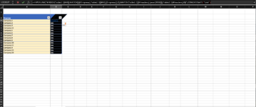
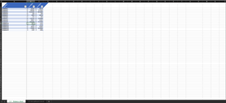
I have two sheets, first of them has a data table with the income of a list of 14 companies during 2018 and 2019. The other sheet I've a data table with a list of these companies and next to the name an hiperlink. When it's selected, it transports you to the cell located in the row of the company.
It's important that both are inside the data table because this is an example file. The original file has 6000 thousand companies and 500 colums of information, therefore it has to have the information well organized, then it's needed to be in data table.
In the table that has the hyperlinks, the formula of the hyperlinks its:
=HYPERLINK("#INDEX(Table2.1[#All];MATCH(A3;Table2.1[[#All];[Empresa]];0);MATCH(Table2.1[[#Headers];[year(2018)]];Table2.1[#Headers];0))";CONCATENATE("Link"))
It works perfectly, but has a little problem. If I decide to sort the table it makes that the cell with the formula that i wrote down continues pointing the "A3" cell even if when sorting it's in another row. The solution would be changing the "A3" for the name of the column.
=HYPERLINK("#INDEX(Table2.1[#All];MATCH([@Empresa];Table2.1[[#All];[Empresa]];0);MATCH(Table2.1[[#Headers];[year(2018)]];Table2.1[#Headers];0))";CONCATENATE("Link"))
But if I do it, the problem is the hyperlink stops to work.... anyone could help me how to solve this problem?
In addition, If I have "A3" in the 3rd row, in 4th should be "A4", etc. but If by mistake I overwrite all column with the formula (don't forget that it's a data table) all cells would point the same cell ej. "A3". Is there any solution for this problem? I suppose that solving the first question would solve this one.
Thanks a lot,
Best regards,


