Hello!
I am looking for a way to do the following:
1. Use a given date in Sheet1
2. Go to Sheet2 and lookup the exact date from Sheet1 in table1, column1
3. If the date isn't listed in the table, end. (aka "")
4. Using date from Column 2, go back to Sheet1
5. If there is data present for the day before and the day after, display a checkmark box (I've already created cell reference for this which is located on Sheet2)
6. If there is data missing on either side of date, end. (aka no checkmark box will be displayed)
Here's what I am thinking so far: =IF(VLOOKUP(U6,Sheet2!$AQ$4:$AS$53,1,FALSE)="XXXX",Sheet2!$AO$3,Sheet2!$AO$4)
**The cell references are my actual references. In order to help me, feel free to change them if it makes it easier for you. The XXXX part is where I am stumped. Essentially the returned value (date if there is one), is then needed to look up back on Sheet1 as a point of reference to see if both adjacent cells have data (time) in them, in order to display the checkmark box in Cell Q15.
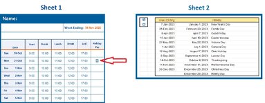
I've attached an illustration with a red arrow to show what I would like to appear if the conditions are met; as described above.
Any better way of doing this? This sounds pretty logical to me but if someone has a better, easier, foolproof way to do this, I'm all ears!
Sheet1
Sheet2
I am looking for a way to do the following:
1. Use a given date in Sheet1
2. Go to Sheet2 and lookup the exact date from Sheet1 in table1, column1
3. If the date isn't listed in the table, end. (aka "")
4. Using date from Column 2, go back to Sheet1
5. If there is data present for the day before and the day after, display a checkmark box (I've already created cell reference for this which is located on Sheet2)
6. If there is data missing on either side of date, end. (aka no checkmark box will be displayed)
Here's what I am thinking so far: =IF(VLOOKUP(U6,Sheet2!$AQ$4:$AS$53,1,FALSE)="XXXX",Sheet2!$AO$3,Sheet2!$AO$4)
**The cell references are my actual references. In order to help me, feel free to change them if it makes it easier for you. The XXXX part is where I am stumped. Essentially the returned value (date if there is one), is then needed to look up back on Sheet1 as a point of reference to see if both adjacent cells have data (time) in them, in order to display the checkmark box in Cell Q15.
I've attached an illustration with a red arrow to show what I would like to appear if the conditions are met; as described above.
Any better way of doing this? This sounds pretty logical to me but if someone has a better, easier, foolproof way to do this, I'm all ears!
Sheet1
Week Ending: | 25-Feb-2023 | |||||||
| Date | Start | Break | Lunch | Break | End | Holiday Pay | ||
| Sun | 17-Feb | 9:00 | 10:00 | 11:00 | 12:00 | 13:00 | ||
| Mon | 18-Feb | 10:00 | 11:00 | 12:00 | 13:00 | 14:00 | Checkmark Box | |
| Tue | 19-Feb | 11:00 | 12:00 | 13:00 | 14:00 | 15:00 | ||
| Wed | 20-Feb | 12:00 | 13:00 | 14:00 | 15:00 | 16:00 | ||
| Thu | 21-Feb | 13:00 | 14:00 | 15:00 | 16:00 | 17:00 | ||
| Fri | 22-Feb | 14:00 | 15:00 | 16:00 | 17:00 | 18:00 | ||
| Sat | 23-Feb | 15:00 | 16:00 | 17:00 | 18:00 | 19:00 |
Sheet2
| Week Ending | Holiday | Checkmark Box Checked | ||
| 31-Dec-2022 | 25-Dec | Christmas Day | Checkmark Box Unchecked | |
| 7-Jan-2023 | 1-Jan | New Year’s Day | ||
| 25-Feb-2023 | 20-Feb | Family Day | ||
| 8-Apr-2023 | 7-Apr | Good Friday | ||
| 15-Apr-2023 | 10-Apr | Easter Monday | ||
| 27-May-2023 | 22-May | Victoria Day | ||
| 1-Jul-2023 | 1-Jul | Canada Day | ||
| 12-Aug-2023 | 7-Aug | Civic Holiday | ||
| 9-Sep-2023 | 4-Sep | Labour Day | ||
| 14-Oct-2023 | 9-Oct | Thanksgiving | ||
| 11-Nov-2023 | 11-Nov | Remembrance Day | ||
| 30-Dec-2023 | 25-Dec | Christmas Day |


