How to Use VLOOKUP to Copy Data Between Sheets Based on a Code?

[happydz]

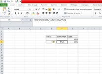
Hello everyone,I'm currently working on an Excel project where I need to copy data from one sheet to another using the VLOOKUP function. I have two sheets:

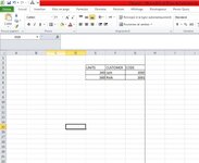
• Sheet1contains the following columns:
  • Column G: CODE
  • Column F: CUSTOMER
  • Column E: UNITS

I want to retrieve the CUSTOMER name based on a specific CODE. For example, when I enter the code 1001 in cell G5 of my second sheet, I want to use VLOOKUP to automatically fill in the corresponding CUSTOMER name in cell F5.Here’s the formula I tried:
F5 =RECHERCHEV(G5,Feuil1!E3:G5,2,FAUX)

However, I keep getting the #N/A error.I've checked that:

• The CODE exists in Sheet1.
• The range is correctly defined.
• There are no leading or trailing spaces in the CODE or CUSTOMER fields.

I’ve attached screenshots of both sheets for reference. Any help or suggestions on how to resolve this issue would be greatly appreciated!Thank you in advance for your assistance!

 

[Umma123]

It sounds like your problem may be with the range you are referencing. The range in your VLOOKUP should start with the column with the lookup value (CODE in Column G) and include the CUSTOMER column. Try updating your thread:
=VLOOKUP(G5,Sheet1!G3:F100,2,FALSE)
If this still doesn’t work, make sure your CODE column is formatted exactly the same on both documents (e.g. as text or numbers). When I had a similar problem, the SkySuite AI was quick to flag formatting inconsistencies I had overlooked and suggested corrections.

 

[etaf]

Are you still using 2010 version of excel
F5 =RECHERCHEV(G5,Feuil1!E3:G5,2,FAUX)
I guess in UK would be
=VLOOKUP(G5,Sheet1!E3:G5,2,FALSE)
so you are only looking in rows 3,4 & 5
looking in column E range row 3 to 5 for a match with G5
if a match found then return the 2nd column starting from E
so thats column F

 

[Alex Blakenburg]

Unless I am missing something here, you are trying to retrieve a value (from col F) to the left of the value you are looking up (col G). VLookup can't do that without introducing a work around, so it is simpler just to use Index Match.

eg

Book2
	E	F	G
3	UNITS	CUSTOMER	CODE
4		#N/A	1003
5		Nick	1001
Sheet2

Cell Formulas
Range	Formula
F4:F5	F4	=INDEX(Sheet1!$F$4:$F$5,MATCH(G4,Sheet1!$G$4:$G$5,0),1)